3.2. Differentiation and Critical Points#
3.2.1. Learning Goals:#
After working through these notes, you will be able to:
Determine critical points for polynomial functions of one variable
Determine critical points for exponential and logarithmic functions
Determine critical points for composite functions
3.2.2. Coding concepts:#
The following coding concepts are used in this notebook:
3.2.3. Critical Points#
Critical points of a function are local maxima or minima in the function. For example, see the 1D function plotted below and the identification of the critical points.
Show code cell source
import matplotlib.pyplot as plt
import numpy as np
%matplotlib inline
# setup plot
fontsize=14
fig = plt.figure(figsize=(4,4), dpi= 120, facecolor='w', edgecolor='k')
plt.grid(which='major', axis='both', color='#808080', linestyle='--')
plt.xlabel("$x$",size=fontsize)
plt.ylabel("$f(x)$",size=fontsize)
x = np.arange(-0.5,2.65,0.1)
def f(x):
    return 2*x**3 - 6.5*x**2 + 5*x + 11
plt.plot(x,f(x),lw=2,c='k')
crit_x = np.roots([6,-13,5])
plt.scatter(crit_x[1],f(crit_x[1]),c="tab:red",s=30)
plt.annotate("Maximum", xy=(crit_x[1],f(crit_x[1])+0.25), color="tab:red",fontsize=fontsize)
plt.scatter(crit_x[0],f(crit_x[0]),c="tab:blue",s=30)
plt.annotate("Minimum", xy=(crit_x[0],f(crit_x[0])-0.75), color="tab:blue",fontsize=fontsize)
plt.tight_layout();
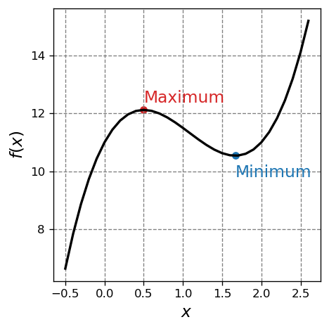
The determination of critical points of functions of one or more variables is fundamental to various aspects of physical chemistry. In these notes, I will present the basic approach for determining critical points of functions of known analytical form and then go through how to differentiate common functions.
The critical points of one dimensional functions are the local maxima and minima of this function. The \(x\) values of these points are determined by setting the derivative of the function to zero and solving for the \(x\) value(s). The dependent values are then determined by plugging in these \(x\) values.
Consider the example below.
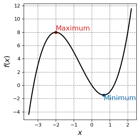
3.2.3.1. Example: Determining Critical Points of a Polynomial#
Determine the critical points of the function
I start by plotting the function.
Show code cell source
import matplotlib.pyplot as plt
import numpy as np
%matplotlib inline
# setup plot
fontsize=14
fig = plt.figure(figsize=(4,4), dpi= 120, facecolor='w', edgecolor='k')
plt.grid(which='major', axis='both', color='#808080', linestyle='--')
plt.xlabel("$x$",size=fontsize)
plt.ylabel("$f(x)$",size=fontsize)
x = np.arange(-3.5,2.25,0.1)
def f(x):
    return x**3 + 2*x**2 -4*x
plt.plot(x,f(x),lw=2,c='k')
crit_x = np.roots([3,4,-4])
plt.scatter(crit_x[0],f(crit_x[0]),c="tab:red",s=30)
plt.annotate("Maximum", xy=(crit_x[0],f(crit_x[0])+0.25), color="tab:red",fontsize=fontsize)
plt.scatter(crit_x[1],f(crit_x[1]),c="tab:blue",s=30)
plt.annotate("Minimum", xy=(crit_x[1],f(crit_x[1])-0.75), color="tab:blue",fontsize=fontsize)
plt.tight_layout();
To determine the critical points, we start by determining the derivative of \(f\) with respect to \(x\)
We determine the \(x\) values of the critical points (there will be two since the derivative is a quadratic and thus will have two roots), we determine the roots of the derivative equation. That is we set the derivative to zero and solve for \(x\):
This can be solved in various ways: (1) the quadratic formula, (2) factoring, when possible, and/or (3) using a calculator to solve for the roots. I will use the numpy roots routine in the code snippet below.
print("Roots:", np.roots([3,4,-4]))
Roots: [-2. 0.66666667]
From the results above we see that the roots of the derivative equation are:
In order to find the f(x) values at these critical points we plug the above \(x\) values into \(f(x)\) (careful not to plug into \(f'(x)\) and also be careful of negative signs):
So, we would report the critical points as \((-2,8)\) and \((\frac{2}{3},-1.48)\).
print(np.roots([3,4,-4]),f(np.roots([3,4,-4])))
[-2. 0.66666667] [ 8. -1.48148148]
3.2.4. Derivatives of common functions#
3.2.4.1. Polynomials#
Derivatives of polynomials show up regulary. These can be determined by the basic rule:
Or, more generally, if we have a polynomial function with a constant, \(A\), in front of \(x\) we have
3.2.5. Rules for Differentiation of Composite Functions#
3.2.5.1. Addition of Functions#
Differentiation of a composite function that is a sum of two functions is just the sum of the derivative of those two functions. This can be written as
This rule comes up all the time when differentiating polynomials. Example:
3.2.5.2. Product Rule#
The derivative of a composite function that is a product of two functions is not as straightforward as the derivative of a function that is a sum of two functions. The product rule for differentiation can be written as
This rule also comes up regularly. Here is an example of its use:
3.2.5.3. The Chain Rule#
A composite function that cannot be written as a simple product or sum of two other functions, such as the log of a polynomial, must be differentiated using the chain rule. The chain rule can be thought of in various ways but I write it here as
Here is an example
import numpy as np
np.roots([6,-2])
array([0.33333333])
3*(1/3)**2-2*1/3+1
0.6666666666666667