4.2.4. Partition Function for a Monatomic Ideal Gas

4.2.4.1. Motivation

We have already seen and used the partition function for an ideal gas in practice problems. Here, we will derive the form of the partition function for a monatomic ideal gas given the quantized translational energy.

4.2.4.2. Learning Goals

After reading these notes, students should be able to:

1. Recognize that whenever you can write the energy of a system as a sum of independent contributions, the partition function is separable as a product of these same contributions

2. Recognize the translational molecular partition function

3. Understand the steps to go from translational energy to a translational partition function

4.2.4.3. Coding Concepts

The following coding concepts are used in this notebook:

1. Variables

2. Functions

3. Plotting with matplotlib

4. Numeric Integration

4.2.4.4. Energy of a Monatomic Ideal Gas

The energy of an ideal gas with constant number of particles, \(N\), volume, \(V\), and temperature, \(T\), is a sum of energies of individual ideal gas particles. A macroscopic state, \(j\), is a sum of particle energies in that particular macroscopic state

(4.89)\[\begin{equation} E_j = \sum_{i=1}^N \epsilon_{i,j}, \end{equation}\]

where \(\epsilon_{i,j}\) denotes the energy of particle \(i\) in macroscopic state \(j\).

Given that we are considering our system to be a monatomic ideal gas, only the translational energy of each particle matters. Quantum mechanics gives this to be

(4.90)\[\begin{equation} \epsilon_{i,j} = \frac{h^2}{8ma^2}\left(n_{x,i,j}^2+n_{y,i,j}^2+n_{z,i,j}^2\right), \end{equation}\]

where \(h\) is Planck’s constant, \(m\) is the mass of the particle and \(a=V^{1/3}\). Each macroscopic state will be differentiated by a the values of \(n_x, n_y, n_z\) taken on for each particle, so \(j\) is actually a list of specific values of \((n_{x,1},n_{y,1},n_{z,1},n_{x,2},..,n_{z,N})\). All macroscopic states will be accounted for by all possible combinations of \(n_x, n_y, n_z\) for each particle. Obviously, the number of possible states will thus be infinitely large.

4.2.4.5. The Canonical Partition Function of an Ideal Gas

The canonical partition function for a monatomic ideal gas is

(4.91)\[\begin{eqnarray} Q &=& \sum_{n_{x,1} = 1,2.., n_{y,1} = 1,2.., .., n_{z,N}=1,2..} e^{-\beta E_{n_{x,1},n_{y,1},..,n_{z,N}}} \\ &=& \sum_j e^{-\beta E_j} \\ &=& \sum_j e^{-\beta \sum_{i=1}^N \epsilon_{i,j}} \\ &=& \sum_j e^{-\beta \epsilon_{1,j}}e^{-\beta \epsilon_{2,j}}...e^{-\beta \epsilon_{N,j}} \end{eqnarray}\]

This can be further simplified by recognizing that the sum can be distributed over the product. Here I will just do it but we will see an example of this later.

(4.92)\[\begin{eqnarray} Q &=& \sum_{n_{x,1},n_{y,1},n_{z,1}} e^{-\beta \epsilon_{1,n_{x,1},n_{y,1},n_{z,1}}}\sum_{n_{x,2},n_{y,2},n_{z,2}}e^{-\beta \epsilon_{2,n_{x,1},n_{y,1},n_{z,1}}}...\sum_{n_{x,N},n_{y,N},n_{z,N}}e^{-\beta \epsilon_{N,n_{x,1},n_{y,1},n_{z,1}}} \\ &=& \prod_{i=1}^N \sum_{n_{x,i},n_{y,i},n_{z,i}} e^{-\beta \epsilon_{1,n_{x,i},n_{y,i},n_{z,i}}} \\ &=& \prod_{i=1}^N q_i, \end{eqnarray}\]

where the notation \(\prod_{i=1}^N\) denotes the product of the argument in analogy to \(\sum\) indicating a sum and \(q_i=\sum_{n_{x,i},n_{y,i},n_{z,i}} e^{-\beta \epsilon_{1,j}}\) denotes a molecular partition function for particle \(i\).

The final steps in the derivation arise from the stiplulation that all particles be identical and indistinguishable. This has the following two results:

1. All \(q_i\) are identical and thus \(\prod_{i=1}^N q_i = q^N\)

2. The particle index \(i\) is arbitrary and thus swapping two particles (e.g. particles 2 and 4) should have no affect on the final result. This leads to an overcounting of \(N!\) per state.

Taking these two aspects into account we get:

(4.93)\[\begin{eqnarray} Q &=& \frac{q^N}{N!} \end{eqnarray}\]

4.2.4.6. Example: Three Ideal Gas Particles

Consider a system of three indistinguishable ideal gas particles held at constant \(V\) and \(T\). Each particle can take on two energy levels denoted \(\epsilon_1\) and \(\epsilon_2\).

1. Write out all possible energy levels of the system.

2. Demonstrate that \(Q \approx \frac{q^N}{N!}\) for this system.

4.2.4.6.1. 1. Write out all possible energy levels

The energy of the system is given as

(4.94)\[\begin{eqnarray} E_j &=& \sum_i \epsilon_{j,i} \\ &=& \epsilon_{j,1} + \epsilon_{j,2} + \epsilon_{j,3}, \end{eqnarray}\]

where here \(j\) is as an ordered triplet, \(j = (1,2,2)\) for example, denoting the states of the three particles.

Each particle can take on one of two energy levels thus yielding a total of \(2^3=8\) possibilities

(4.95)\[\begin{eqnarray} E_1 = \epsilon_{1,1} + \epsilon_{1,2} + \epsilon_{1,3} &=& 3\epsilon_1 \\ E_2 = \epsilon_{2,1} + \epsilon_{1,2} + \epsilon_{1,3} &=& 2\epsilon_1 + \epsilon_2 \\ E_3 = \epsilon_{1,1} + \epsilon_{2,2} + \epsilon_{1,3} &=& 2\epsilon_1 + \epsilon_2 \\ E_4 = \epsilon_{1,1} + \epsilon_{1,2} + \epsilon_{2,3} &=& 2\epsilon_1 + \epsilon_2 \\ E_5 = \epsilon_{2,1} + \epsilon_{2,2} + \epsilon_{1,3} &=& \epsilon_1 + 2\epsilon_2 \\ E_6 = \epsilon_{2,1} + \epsilon_{1,2} + \epsilon_{2,3} &=& \epsilon_1 + 2\epsilon_2 \\ E_7 = \epsilon_{1,1} + \epsilon_{2,2} + \epsilon_{2,3} &=& \epsilon_1 + 2\epsilon_2 \\ E_8 = \epsilon_{2,1} + \epsilon_{2,2} + \epsilon_{2,3} &=& 3\epsilon_2 \\ \end{eqnarray}\]

Notice, however, that there are really only four different values for the total energy. Additionally, since the particles are indistinguishable, each of the substates of the four different energy levels are indistinguishable. So really we have the following four system energy levels:

(4.96)\[\begin{eqnarray} E_1 &=& 3\epsilon_1 \\ E_2 &=& 2\epsilon_1 + \epsilon_2 \\ E_3 &=& \epsilon_1 + 2\epsilon_2 \\ E_4 &=& 3\epsilon_2 \\ \end{eqnarray}\]

4.2.4.6.2. 2. Demonstrate \(Q \approx \frac{q^N}{N!}\).

We have four system energy levels and can thus just write out the overall partition function for this system

(4.97)\[\begin{eqnarray} Q &=& e^{-\beta 3\epsilon_1} + e^{-\beta (2\epsilon_1 + \epsilon_2)} + e^{-\beta (\epsilon_1 + 2\epsilon_2)} + e^{-\beta 3\epsilon_2} \\ &=& e^{-\beta (\epsilon_{1,1} + \epsilon_{1,2} + \epsilon_{1,3})} + \frac{1}{3}\left( e^{-\beta (\epsilon_{2,1} + \epsilon_{1,2} + \epsilon_{1,3})} + e^{-\beta (\epsilon_{1,1} + \epsilon_{2,2} + \epsilon_{1,3})} + e^{-\beta (\epsilon_{1,1} + \epsilon_{1,2} + \epsilon_{2,3})}\right) + \frac{1}{3}\left( e^{-\beta (\epsilon_{2,1} + \epsilon_{2,2} + \epsilon_{1,3})} + e^{-\beta (\epsilon_{2,1} + \epsilon_{1,2} + \epsilon_{2,3})} + e^{-\beta (\epsilon_{1,1} + \epsilon_{2,2} + \epsilon_{2,3})}\right) + e^{-\beta (\epsilon_{2,1} + \epsilon_{2,2} + \epsilon_{2,3})} \\ &=& \frac{1}{3}\left(e^{-\beta \epsilon_{1,1}} + e^{-\beta \epsilon_{2,1}}\right) \left(e^{-\beta \epsilon_{1,2}} + e^{-\beta \epsilon_{2,2}}\right)\left(e^{-\beta \epsilon_{1,3}} + e^{-\beta \epsilon_{2,3}}\right) + \frac{2}{3}\left(e^{-\beta (\epsilon_{1,1} + \epsilon_{1,2} + \epsilon_{1,3})} + e^{-\beta (\epsilon_{2,1} + \epsilon_{2,2} + \epsilon_{2,3})}\right)\\ &\approx& \frac{1}{3}\sum_{j=1}^{2} e^{-\beta \epsilon_{j,1}}\sum_{j=1}^{2} e^{-\beta \epsilon_{j,2}}\sum_{j=1}^{2} e^{-\beta \epsilon_{j,3}} \\ &=& \frac{1}{3}q_1 \cdot q_2 \cdot q_3 \\ &=& \frac{1}{3}q^3 \\ &\approx& \frac{q^N}{N!} \end{eqnarray}\]

A few comments on this. First, we see that we do not get, exactly, \(Q = q^N/N!\). That is because the factorial correction for indistinguishable particles is an approximation. It is technically only valid for states in which all particles occupy different states (not possible in this particular example). This is deemed a good approximation because at high enough temperature (or small enough spaced energy levels), it is likely that the particles will occupy different states.

4.2.4.7. Achieving an Analytic Solution for the Translational Partition Function

So far we have demonstrated that, for an ideal gas, we have a Canonical partition function of the form

(4.98)\[\begin{equation} Q = \frac{q^N}{N!}, \end{equation}\]

where \(q = \sum_je^{-\beta \epsilon_j}\) is termed the molecular partition function with molecular energy \(\epsilon_j\) for molecular state \(j\). For a monatomic ideal gas only the translational energy of each particle comes into play and thus

(4.99)\[\begin{equation} \epsilon_{n_x,n_y,n_z} = \frac{h^2}{8ma^2}\left(n_x^2 + n_y^2 + n_z^2\right), \quad n_x,n_y,n_z=1, 2, ... \end{equation}\]

The goal now is to plug in the energy equation into \(q\) and derive an analytic expression for the resulting sum (and ultimately plug this result back into the above equation for \(Q\)).

We start by simply plugging in the energy into \(q\)

(4.100)\[\begin{eqnarray} q_{trans} &=& \sum_{n_x,n_y,n_z} e^{-\beta \epsilon_{n_x,n_y,n_z}} \\ &=& \sum_{n_x=1}^{\infty}\sum_{n_y=1}^{\infty}\sum_{n_z=1}^{\infty} \exp\left[ \frac{-\beta h^2}{8ma^2}\left(n_x^2 + n_y^2 + n_z^2\right) \right] \\ &=& \sum_{n_x=1}^{\infty}\exp\left(\frac{-\beta h^2n_x^2}{8ma^2}\right)\sum_{n_y=1}^{\infty}\exp\left(\frac{-\beta h^2n_y^2}{8ma^2}\right)\sum_{n_z=1}^{\infty} \exp\left(\frac{-\beta h^2n_z^2}{8ma^2} \right) \\ &=& \left[ \sum_{n=1}^{\infty}\exp\left(\frac{-\beta h^2n^2}{8ma^2}\right) \right]^3 \end{eqnarray}\]

Where I have now labeled the molecular partition function \(q_{trans}\) to denote that it is for the translational component of the energy. We now need to evaluate the sum inside the square brackets.

In order to evaluate this sum we will make the approximation that the spacing of the translational energy levels is very small relative to \(k_BT\) and thus we can approximate the sum of quantum number \(n\) as an integral over continuous variable \(n\):

(4.101)\[\begin{eqnarray} \sum_{n=1}^{\infty}\exp\left(\frac{-\beta h^2n^2}{8ma^2}\right) \approx \int_0^{\infty} e^{\frac{-\beta h^2n^2}.{8ma^2}}dn \end{eqnarray}\]

Recall from our section on continuous probability that

(4.102)\[\begin{eqnarray} \int_0^\infty e^{-\alpha x^2}dx = \sqrt{\frac{\pi}{4\alpha}} \end{eqnarray}\]

Thus we get that

(4.103)\[\begin{eqnarray} \int_0^{\infty} e^{\frac{-\beta h^2n^2}{8ma^2}}dn &=& \left( \frac{8\pi m a^2}{4\beta h^2} \right)^{1/2} \\ &=& \left( \frac{2\pi m k_BT}{ h^2} \right)^{1/2}a \end{eqnarray}\]

Plugging this back into \(q_{trans}\) yields

(4.104)\[\begin{eqnarray} q_{trans} &=& \left[ \left( \frac{2\pi m k_BT}{ h^2} \right)^{1/2}a \right]^3\\ &=& \left( \frac{2\pi m k_BT}{ h^2} \right)^{3/2}a^3 \\ &=& \left( \frac{2\pi m k_BT}{ h^2} \right)^{3/2}V \end{eqnarray}\]

where the last equality comes from the fact that \(a=V^{1/3}\).

Finally, we can plug this back into the equation for \(Q\) to get the final expression for the partition function of a monatomic ideal gas

(4.105)\[\begin{equation} Q = \frac{\left( \frac{2\pi m k_BT}{ h^2} \right)^{3N/2}V^N}{N!} \end{equation}\]

4.2.4.8. Example 1: Integration vs Summation

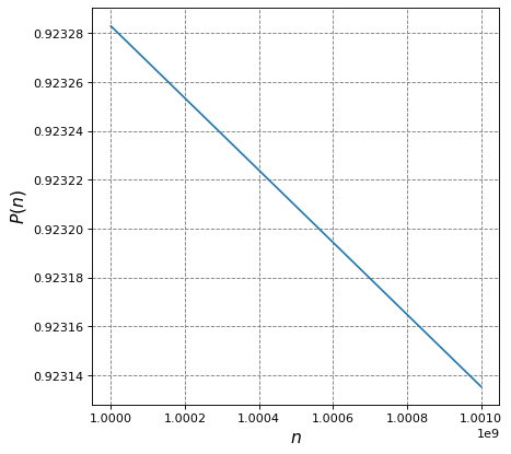
Consider the following function of \(n\):

(4.106)\[\begin{equation} f(n) = \exp\left( \frac{-\beta h^2n^2}{8ma^2} \right) \end{equation}\]

Evaluate the following two functions over domain \(1\times10^9 \leq n \leq 1.001\times10^9\) and with \(m=1\) amu, \(T=300\) K, and \(a=1\) dm.

(4.107)\[\begin{equation} \sum_{n=1\times10^9}^{1.001\times10^9} f(n) \end{equation}\]

and

(4.108)\[\begin{equation} \int_{1\times10^9}^{1.001\times10^9} f(n)dn \end{equation}\]

import numpy as np
T = 300
kB = 1.380649e-23 # m2 kg s-2 K-1 
m = 1.66e-26  # Kg 
a = 1e-1 # m 
h = 6.62607015e-34 # m2 kg / s 
prefactor = h**2/(8*m*a**2*kB*T)
print(prefactor)
def f(n):
    return np.exp(-prefactor * n**2)

7.981958150357973e-20

from scipy.integrate import quad
n = np.arange(1e9,1.001e9,1)
summation = np.sum(f(n))
numeric_integral = quad(f,1e9,1.001e9)[0]
print("Sum:", summation)
print("Integral:", numeric_integral)
print("Percent Error:", np.abs(summation-numeric_integral)/summation*100)

Sum: 923209.1920522513
Integral: 923209.1919785243
Percent Error: 7.985945991538972e-09

import matplotlib.pyplot as plt
%matplotlib inline
# setup plot 
fontsize=14
fig = plt.figure(figsize=(6,6), dpi= 80, facecolor='w', edgecolor='k')
ax = plt.subplot(111)
ax.grid(b=True, which='major', axis='both', color='#808080', linestyle='--')
ax.set_xlabel("$n$",size=fontsize)
ax.set_ylabel("$P(n)$",size=fontsize)
plt.plot(n,f(n))

[<matplotlib.lines.Line2D at 0x7facf27bdf40>]

4.2.4.9. Example 2: Average \(n\)

Consider a monatomic ideal gas particle in 1D with m = 1.66x10\(^{-26}\) kg, a = 1x10\(^{-6}\) m, and T=10 K. What is the average value of the translational quantum number \(n\) assuming that it is continuous.

Some relevant equations, first the translational partition function in 1D

(4.109)\[\begin{equation} q_{}\left(a,T\right)=\left(\frac{2\pi mk_{B}T}{h^2}\right)^{\frac{1}{2}}a \end{equation}\]

Next a potentially useful integral

(4.110)\[\begin{equation} \int_0^{\infty}ne^{-\alpha n^2}dn=\frac{1}{2\alpha} \end{equation}\]

We will also need that:

(4.111)\[\begin{eqnarray} h &=& 6.626\times10^{-34} \quad m^2\cdot kg \cdot s^{-1}\\ k_B &=& 1.381 \times10^{-23} \quad m^2\cdot kg \cdot s^{-2} \cdot K^{-1}\\ \epsilon_n &=& \frac{h^2n^2}{8ma^2} \end{eqnarray}\]

where the equation for \(\epsilon_n\) is the particle in a box energy for 1D.

The problem asks for the average \(n\), for continuous variable \(n\). This can be written as a standard weighted average

(4.112)\[\begin{equation} \langle n \rangle = \int_0^\infty nP(n)dn, \end{equation}\]

where \(P(n)\) is the probability density of variable \(n\). \(P(n)\) can be determined as the ratio of the Boltzmann factor of a particular \(n\) releative to the parition function, \(q\),

(4.113)\[\begin{eqnarray} P(n) &=& \frac{e^{-\beta \epsilon_n}}{q} \\ &=& \frac{e^{-\beta \frac{h^2n^2}{8ma^2}}}{q} \end{eqnarray}\]

Plug this equation into the integral for \(\langle n \rangle\) yields

(4.114)\[\begin{eqnarray} \langle n \rangle &=& \int_0^\infty nP(n)dn \\ &=& \int_0^\infty n frac{e^{-\beta \frac{h^2n^2}{8ma^2}}}{q} dn \\ &=& \frac{1}{q} \int_0^\infty n e^{-\beta \frac{h^2n^2}{8ma^2}} dn \end{eqnarray}\]

Now, let \(\alpha = \beta \frac{h^2}{8ma^2}\) yields

(4.115)\[\begin{eqnarray} \langle n \rangle &=& \frac{1}{q} \int_0^\infty n e^{-\alpha n^2} dn \\ &=& \frac{1}{q} \frac{1}{2\alpha} \\ &=& \frac{1}{q} \frac{8ma^2}{2\beta h^2} \\ &=& \frac{1}{q} \frac{4ma^2k_BT}{ h^2} \end{eqnarray}\]

Now we can either plug in numbers or put in \(q\) as variables, simplify and then plug in numbers. Here I will do that latter:

(4.116)\[\begin{eqnarray} \langle n \rangle &=& \frac{1}{q} \frac{4ma^2k_BT}{ h^2} \\ &=& \left(\frac{2\pi mk_{B}T}{h^2}\right)^{\frac{-1}{2}}a^{-1} \frac{4ma^2k_BT}{ h^2} \\ &=& \frac{4\sqrt{mk_BT}a}{ \sqrt{2\pi}h} \\ &=& \frac{4a}{h}\sqrt{\frac{mk_BT}{2\pi}} \end{eqnarray}\]

T = 10
kB = 1.380649e-23 # m2 kg s-2 K-1 
m = 1.66e-26  # Kg 
a = 1e-6 # m 
h = 6.62607015e-34 # m2 kg / s 
print("<n> = ", np.round(4*a/h*np.sqrt(m*kB*T/(2*np.pi)),2))

<n> =  3645.94

4.2.4.10. Example 3: Order of magnitude of \(n\)

Consider a monatomic ideal gas particle in 1D with m = 1.66x10\(^{-26}\) kg, a = 1x10\(^{-6}\) m, and T=10 K. What is the order of magnitude of the typical of the translational quantum number \(n\) assuming that it is continuous?

Additional information you will need:

(4.117)\[\begin{eqnarray} h &=& 6.626\times10^{-34} \quad m^2\cdot kg \cdot s^{-1}\\ k_B &=& 1.381 \times10^{-23} \quad m^2\cdot kg \cdot s^{-2} \cdot K^{-1}\\ \epsilon_n &=& \frac{h^2n^2}{8ma^2} \\ \langle \epsilon_{1D} \rangle &=& \frac{1}{2}k_BT \end{eqnarray}\]

To address this problem one could:

1. Compute \(\langle n \rangle\) as we did in the previous example

2. Determine the value of \(n\) that corresponds to \(\langle \epsilon \rangle\).

We will do option 2 here.

(4.118)\[\begin{eqnarray} \langle \epsilon_{1D} \rangle &=& \frac{1}{2}k_BT \\ &=& \frac{h^2n_{typical}^2}{8ma^2} \\ \Rightarrow n_{typical} &=& \sqrt{\frac{4ma^2k_BT}{h^2}} \end{eqnarray}\]

We plug-in numbers below using a code snippet.

T = 10 # K
kB = 1.380649e-23 # m2 kg s-2 K-1 
m = 1.66e-26  # Kg 
a = 1e-6 # m 
h = 6.62607015e-34 # m2 kg / s 
print("n_typical = ", np.round(np.sqrt(4*m*a**2*kB*T/h**2),2))

n_typical =  4569.51