The Pressure and Temperature Dependence of the Gibbs Energy

4.3.15. The Pressure and Temperature Dependence of the Gibbs Energy#

4.3.15.1. Learning Goals#

After reading and understanding these notes, you will be able to

Derive the relationship between Gibbs free energy and pressure for an ideal gas
Express the fugacity of a real gas in terms of a virial expansion
Derive the relationship between Gibbs free energy and temperature (Gibbs-Helmholtz equation)
Calculate \(G(T)\) from data on heat capacity and phase transitions for a substance.

4.3.15.2. Coding Concepts#

The following coding concepts are used in this notebook:

4.3.15.3. Differential Form of the Gibbs Energy#

The differential form of the Gibbs energy as a function of only two variables is

(4.359)#\[\begin{equation} dG = -SdT + VdP \end{equation}\]

which implies the following first derivative relationships

(4.360)#\[\begin{eqnarray} \left( \frac{\partial G}{\partial T} \right)_P &=& -S \\ \left( \frac{\partial G}{\partial P} \right)_T &=& V \end{eqnarray}\]

These two equations can be used to determine the pressure and temperature dependence of \( G\).

4.3.15.4. Pressure Dependence of \(G\)#

The partial derivative relationship can be used to determine the pressure dependence of \( G\). The derivation is as follows

(4.361)#\[\begin{eqnarray} \left( \frac{\partial G}{\partial P} \right)_T &=& V \\ \Rightarrow dG &=& VdP \quad\text{constant T} \\ \Rightarrow \Delta G &=& \int_{P_1}^{P_2}VdP \quad\text{constant T} \end{eqnarray}\]

For an ideal gas we have \(V = \frac{nRT}{P}\) yielding

(4.362)#\[\begin{eqnarray} \Delta G &=& \int_{P_1}^{P_2}\frac{nRT}{P}dP \quad\text{constant T} \\ &=& nRT\ln\frac{P_2}{P_1} \end{eqnarray}\]

\(P = 1\) bar is used as a standard reference so if we set that as the initial state we get

(4.363)#\[\begin{eqnarray} \Delta G &=& G(T,P_2) - G(T,1 \text{bar}) &=& nRT\ln\frac{P_2}{1 \text{bar}} \\ \Rightarrow G(T,P_2) &=& G^\circ(T) + nRT\ln\frac{P_2}{1 \text{bar}} \end{eqnarray}\]

where \(G^\circ(T)\) is the Gibbs free energy of the substance at \(P=1\) bar and the temperature of interest.

The logarithmic dendence of \(G\) on \(P\) is an entirely entropic effect.

The equation above is most commonly written as

(4.364)#\[\begin{eqnarray} G(T,P) &=& G^\circ(T) + nRT\ln\frac{P}{P^\circ} \end{eqnarray}\]

4.3.15.4.1. For a Non-Ideal Gas#

The above equation was derived for an ideal gas. It is useful to derive a similar expression for non-ideal gasses. Here we will use the virial expansion for the equation of state of general non-ideal gas. This has the form

(4.365)#\[\begin{equation} \frac{P\bar{V}}{RT} = 1 + B(T)P + C(T)P^2 + ... \end{equation}\]

If we substitute this equation of state in for the volume in the above derivation we get

(4.366)#\[\begin{equation} \int_{P^{id}}^Pd\bar{G} = RT\int_{P^{id}}^P\frac{dP'}{P'} + RTB(T)\int_{P^{id}}^PdP'+ RTC(T)\int_{P^{id}}^PP'dP'+... \end{equation}\]

Doing the integrtion yields

(4.367)#\[\begin{equation} \bar{G}(T,P) = \bar{G}(T,P^{id}) + RT\ln\frac{P}{P^{id}} + RTB(T)P + \frac{RTC(T)P^2}{2} + ... \end{equation}\]

This can be rewritten as

(4.368)#\[\begin{equation} \bar{G}(T,P) = G^\circ(T)+ RT \ln\frac{f(P,T)}{f^\circ} \end{equation}\]

where \(f\) is called the fugacity and is given by (for virial expansion)

(4.369)#\[\begin{equation} \frac{f(P,T)}{f^\circ} = \frac{P}{P^\circ}\exp\left[B(T)P + C(T)P^2 + ... \right] \end{equation}\]

It can also be shown that \(f^\circ = P^\circ\)

4.3.15.5. Temperature Dependence of \(G\)#

The partial derivative relationship can be used to determine the temperature dependence of \( G\). The derivation is as follows

(4.370)#\[\begin{eqnarray} \left( \frac{\partial G}{\partial T} \right)_P &=& -S \\ \Rightarrow dG &=& -SdT \quad\text{constant P} \\ \Rightarrow \Delta G &=& -\int_{T_1}^{T_2}SdP \quad\text{constant P} \end{eqnarray}\]

Unlike for the pressure dependence, this does not get us far because we cannot typically measure \(S\). Rather, we will do the following manipulations

(4.371)#\[\begin{eqnarray} \left( \frac{\partial G}{\partial T} \right)_P &=& -S \\ \Rightarrow \frac{1}{T}\left( \frac{\partial G}{\partial T}\right)_P &=& -\frac{S}{T} \\ \Rightarrow \left( \frac{\partial \frac{G}{T}}{\partial T}\right)_P + \frac{G}{T^2} &=& -\frac{S}{T} \\ \Rightarrow \left( \frac{\partial \frac{G}{T}}{\partial T}\right)_P &=& -\frac{G+TS}{T^2} \\ \Rightarrow \left( \frac{\partial \frac{G}{T}}{\partial T}\right)_P &=& -\frac{H}{T^2} \end{eqnarray}\]

This last equation is called the Gibbs-Helmholtz equation. We will use it in subsequent parts of this course to investigate the temperature dependence of the Gibbs free energy of chemical equilibria. Applied to a process, this becomes

(4.372)#\[\begin{eqnarray} \left( \frac{\partial \frac{G}{T}}{\partial T}\right)_P &=& -\frac{\Delta H}{T^2} \end{eqnarray}\]

The implications of this equation are that we can compute the Gibbs free energy of a substance at a given \(T\) from tabulated enthalpy and entropy information. Or, equivalently

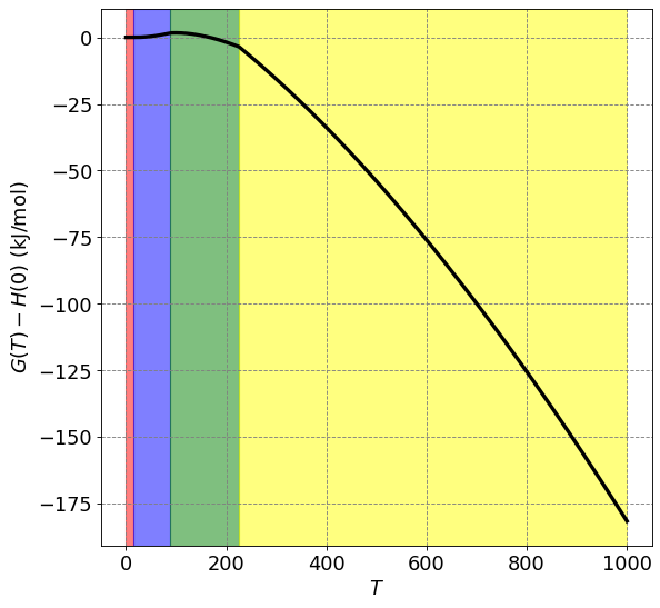
(4.373)#\[\begin{equation} \bar{G}(T) - \bar{H}(0) = \bar{H}(T)-\bar{H}(0) - T\bar{S}(T) \end{equation}\]

4.3.15.5.1. Example: Temperature Dependence of \(G\) for Propene#

Given the following fata for propene, plot \(\bar{G}(T) - \bar{H}(0)\) versus \(T\). (assume ideal gas behavior)

\[\begin{eqnarray*} \bar{C}_p^s &=& R \frac{12\pi^4}{5}\left( \frac{T}{100.}\right)^3 \quad 0 < T < 15 K \\ \bar{C}_p^s &=& R \left(-1.663+ 0.001112T - 9.791\times10^{-4}T^2 + 3.740\times10^{-6}T^3 \right) \quad 15 < T < 87.90 \text{K} \\ \bar{C}_p^l &=& R \left(15.935 - 0.08677T + 4.294\times10^{-4}T^2 - 6.276\times10^{-7}T^3\right) \quad 87.90 < T < 225.46 \text{K} \\ \bar{C}_p^g &=& R \left(1.4970 + 2.266\times10^{-2}T - 5.725\times10^{-6}T^2 \right) \quad 225.46 < T < 1000 \text{K} \end{eqnarray*}\]

and

\[\begin{eqnarray*} T_{fusion} &=& 87.90 \quad \text{K} \\ \Delta \bar{H}_{fusion} &=& 3.00 \quad \text{kJ}\cdot\text{mol}^{-1} \\ T_{vap} &=& 225.46 \quad \text{K} \\ \Delta \bar{H}_{vap} &=& 18.42 \quad \text{kJ}\cdot\text{mol}^{-1} \\ \end{eqnarray*}\]

We want \(\bar{G}(T) - \bar{H}(0)\) which we know to be equal to

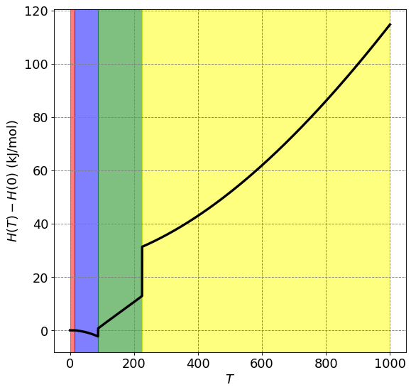
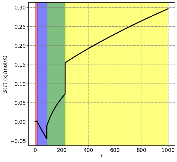
(4.374)#\[\begin{equation} \bar{G}(T) - \bar{H}(0) = \bar{H}(T)-\bar{H}(0) - T\bar{S}(T) \end{equation}\]

So we calculate \(\bar{H}(T)-\bar{H}(0)\) and \(\bar{S}(T)\) separately.

From previous discussions, we know that

(4.375)#\[\begin{eqnarray} \bar{H}(T)-\bar{H}(0) = \Delta H = \int_0^{15} \bar{C}_p^s dT + \int_{15}^{87.90} \bar{C}_p^s dT + \Delta \bar{H}_{fusion} + \int_{87.90}^{225.46}\bar{C}_p^ldT + \Delta \bar{H}_{vap} + \int_{225.46}^{T}\bar{C}_p^gdT \end{eqnarray}\]

Similarly, we know that

(4.376)#\[\begin{eqnarray} \bar{S}(T) = \int_0^{15} \frac{\bar{C}_p^s}{T} dT + \int_{15}^{87.90} \frac{\bar{C}_p^s}{T} dT + \frac{\Delta \bar{H}_{fusion}}{T} + \int_{87.90}^{225.46}\frac{\bar{C}_p^l}{T}dT + \frac{\Delta \bar{H}_{vap}}{T} + \int_{225.46}^{T}\frac{\bar{C}_p^g}{T}dT \end{eqnarray}\]

Below I will use code and numeric integration to make this plot.

import numpy as np
import scipy.integrate as integrate
R = 8.314 # J/K/mol
# heat capacity of first solid state
def cp_s1(T):
    return R*12*np.pi**4/5*(T/100)**3
# heat capacity of second solid state
def cp_s2(T):
    return R*(-1.663 + 0.001112*T - 9.791e-4*T**2 + 3.740e-6*T**3)
# heat capacity of liquid
def cp_l(T):
    return R*(15.935 - 0.08677*T + 4.294e-4*T**2 - 6.276e-7*T**3)
# heat capacity of gass
def cp_g(T):
    return R*(1.4970 + 2.266e-2*T - 5.725e-6*T**2)
int_cp_s1 = integrate.quad(cp_s1,0,15)[0]
print("int 0 to 15", int_cp_s1, "J/mol")
int_cp_s2 = integrate.quad(cp_s2,15,87.90)[0]
print("int 15 to 87.90", int_cp_s2, "J/mol")
int_cp_l = integrate.quad(cp_l,87.90,225.46)[0]
print("int 87.90 to 225.46", int_cp_l, "J/mol")

int 0 to 15 24.599472679272154 J/mol
int 15 to 87.90 -2343.2433212427372 J/mol
int 87.90 to 225.46 12213.373101852707 J/mol

import matplotlib.pyplot as plt
%matplotlib inline
#def f(T)
def H(T_array):
    f = []
    for T in T_array:
        if T<=15:
            f.append(integrate.quad(cp_s1,0,T)[0])
        elif T>15 and T<=87.90:
            f.append(int_cp_s1 + integrate.quad(cp_s2,15,T)[0])
        elif T>87.90 and T<=225.46:
            f.append(int_cp_s1 + int_cp_s2 + 3e3 + integrate.quad(cp_l,87.90,T)[0])
        else:
            f.append(int_cp_s1 + int_cp_s2 + 3e3 + int_cp_l + 18.42e3 + integrate.quad(cp_g,225.46,T)[0])
    return np.array(f)

# setup plot parameters
fontsize=16
fig = plt.figure(figsize=(8,8), dpi= 80, facecolor='w', edgecolor='k')
ax = plt.subplot(111)
ax.grid(b=True, which='major', axis='both', color='#808080', linestyle='--')
ax.set_xlabel("$T$",size=fontsize)
ax.set_ylabel("$H(T) - H(0)$ (kJ/mol)",size=fontsize)
plt.tick_params(axis='both',labelsize=fontsize)
T = np.arange(0.1,1000,0.1)
plt.plot(T,H(T)/1000,lw=3,c='k')
ax.axvspan(0, 15, alpha=0.5, color='red')
ax.axvspan(15, 87.90, alpha=0.5, color='blue')
ax.axvspan(87.90, 225.46, alpha=0.5, color='green')
ax.axvspan(225.46, 1000, alpha=0.5, color='yellow')

<matplotlib.patches.Polygon at 0x7f8c587798b0>

../../_images/e2864a3ff3681703118916793659efba545f867efa4c54cabe0892a644d2218c.png

import numpy as np
import scipy.integrate as integrate
R = 8.314 # J/K/mol
# heat capacity of first solid state
def s_s1(T):
    return cp_s1(T)/T
# heat capacity of second solid state
def s_s2(T):
    return cp_s2(T)/T
# heat capacity of liquid
def s_l(T):
    return cp_l(T)/T
# heat capacity of gass
def s_g(T):
    return cp_g(T)/T
int_s_s1 = integrate.quad(s_s1,0,15)[0]
print("int 0 to 15", int_s_s1, "J/mol/K")
int_s_s2 = integrate.quad(s_s2,15,87.90)[0]
print("int 15 to 87.90", int_s_s2, "J/mol/K")
int_s_l = integrate.quad(s_l,87.90,225.46)[0]
print("int 87.90 to 225.46", int_s_l, "J/mol/K")

int 0 to 15 2.18661979371308 J/mol/K
int 15 to 87.90 -47.300135968020605 J/mol/K
int 87.90 to 225.46 83.74783642272298 J/mol/K

import matplotlib.pyplot as plt
%matplotlib inline
#def f(T)
def S(T_array):
    f = []
    for T in T_array:
        if T<=15:
            f.append(integrate.quad(s_s1,0,T)[0])
        elif T>15 and T<=87.90:
            f.append(int_s_s1 + integrate.quad(s_s2,15,T)[0])
        elif T>87.90 and T<=225.46:
            f.append(int_s_s1 + int_s_s2 + 3e3/87.90 + integrate.quad(s_l,87.90,T)[0])
        else:
            f.append(int_s_s1 + int_s_s2 + 3e3/87.90 + int_s_l + 18.42e3/225.46 + integrate.quad(s_g,225.46,T)[0])
    return np.array(f)

# setup plot parameters
fontsize=16
fig = plt.figure(figsize=(8,8), dpi= 80, facecolor='w', edgecolor='k')
ax = plt.subplot(111)
ax.grid(b=True, which='major', axis='both', color='#808080', linestyle='--')
ax.set_xlabel("$T$",size=fontsize)
ax.set_ylabel("$S(T)$ (kJ/mol/K)",size=fontsize)
plt.tick_params(axis='both',labelsize=fontsize)
T = np.arange(0.1,1000,0.1)
plt.plot(T,S(T)/1000,lw=3,c='k')
ax.axvspan(0, 15, alpha=0.5, color='red')
ax.axvspan(15, 87.90, alpha=0.5, color='blue')
ax.axvspan(87.90, 225.46, alpha=0.5, color='green')
ax.axvspan(225.46, 1000, alpha=0.5, color='yellow')

<matplotlib.patches.Polygon at 0x7f8c885f8fa0>

../../_images/737741b8f3ffc08cab212e192846dbeba4e7b4f67c2be5f3b3f1e80b2f43f441.png

import matplotlib.pyplot as plt
%matplotlib inline
#def G(T)
def G(T):
    return H(T) - T*S(T)

# setup plot parameters
fontsize=16
fig = plt.figure(figsize=(8,8), dpi= 80, facecolor='w', edgecolor='k')
ax = plt.subplot(111)
ax.grid(b=True, which='major', axis='both', color='#808080', linestyle='--')
ax.set_xlabel("$T$",size=fontsize)
ax.set_ylabel("$G(T) - H(0)$ (kJ/mol)",size=fontsize)
plt.tick_params(axis='both',labelsize=fontsize)
T = np.arange(0.1,1000,0.1)
plt.plot(T,G(T)/1000,lw=3,c='k')
ax.axvspan(0, 15, alpha=0.5, color='red')
ax.axvspan(15, 87.90, alpha=0.5, color='blue')
ax.axvspan(87.90, 225.46, alpha=0.5, color='green')
ax.axvspan(225.46, 1000, alpha=0.5, color='yellow')

<matplotlib.patches.Polygon at 0x7f8c78a06c10>

../../_images/06ec80d47d6bbc264e37960dd71e829e7edacc1dfce388658698c86ce744c1a1.png