4.5.20. The H\(_2\) Molecule using the Variational Method in a Minimal Basis#
4.5.20.1. Motivation:#
We will discuss the H\(_2\) molecule in a minimal basis of 1s orbitals on each nucleus.
4.5.20.2. Learning Goals:#
After these notes you will be able to:
Write out the Hamiltonian for the H\(_2\) molecule.
Describe the general behavior of the E vs R curve for the variational solution in the minimal basis
Describe the issue with the dissociation limit of the H\(_2\) molecule in the single determinant picture
Identify possible solutions to deal with the dissociation limit issue.
4.5.20.3. Coding Concepts:#
The following coding concepts are used in this notebook:
4.5.20.4. Background#
The Born-Oppenheimer Hamiltonian for H\(_2\) (in atomic units) looks like
where we label the two nuclei as \(A\) and \(B\) and the two electrons as \(1\) and \(2\) such that \(r_{1A}\) is the distance between nucleus \(A\) and electron 1.
Unlike the case of H\(_2^+\), we have an electron-electron coupling term, \(\frac{1}{r_{12}}\), that makes the Schrodinger equation for this Hamiltonian impossible to solve exactly.
Unsurprisingly, there have been many proposed solutions/approximations to the H\(_2\) molecule. We will investigate the variational solution in the minimal basis of two 1s Slater orbitals on each nucleus. This approximation is essentially the linear combination of atomic orbitals (LCAO) description of the H\(_2\) molecule.
4.5.20.5. What We Want to Know#
We would like to be able to descibe the bond distance, bonding energy, and ideally the dissociation energy of the H\(_2\) molecule. We will see that this latter point is challenging for the simple pictures we will describe. Regardless, the experimental, or target, values for these things are:
The dissociation energy is just \(D_e = E_{min} - (-1)\) Hartree since the ground state energy of a single hydrogen atom is known to be exactly \(-0.5\) Hartree.
There are methods based on the varitiational method with over 10s-100s of terms that can get the experimental energy to within three decimal places (in atomic units). We will not work through those examples but rather a very simple varitiational method with one variational parameter.
4.5.20.6. The Trial Wave Function#
The wave function for H\(_2\) will depend on the position of two electrons. We will denote these positions \(\vec{r}_1\) and \(\vec{r}_2\). We will assume that the wave function is separable into functions of each electron. Additionally, we will assume that each electron sits in a bonding orbital that is made up of two Slater 1s orbitals, like we determined for the H\(_2^+\) molecule.
Written out explcitly, we will posit the following trial wave function:
where \(\sigma_b(\vec{r})\) is the bonding orbital that we determined for H\(_2\) plus in a 1s Slater basis. This can be expressed as
Note that \(r_{1A}\) is the distance from electron one to nucleus \(A\). It is a function of the position of that electron, \(\vec{r}_1\), and position of nucleus \(A\).
We can plug the last equation for the bonding orbital into the trial wave function to achieve
4.5.20.7. Variational Energy for H\(_2\)#
With a trial wave function posited, the next step in the variational procedure is to determine the expectation value of the energy. Because the proposed wave function is normalized this is simply
The procedure to determine this solution is similar to the H\(_2^+\) molecule but the calculus/algebra is just a bit more tedious. Some of the integrals are over two electrons and there are more terms in the Hamiltonian. This is just to say that I will not provide the step-by-step derivation but just provide the answer
where we have seen the functions \(S(R)\), \(J(R)\), and \(K(R)\) from our discussion of the H\(_2^+\) molecule. The new functions \(J'(R)\), \(K'(R)\), and \(L(R)\) all come from two electron integrals. All six of these functions are tabulated below
Function |
Integral |
Solution in H\(_2\) Minimal Basis |
|---|---|---|
\(S(ZR)\) |
\(S(ZR) = \left\langle \phi_{1s_A} \mid \phi_{1s_B} \right\rangle\) |
\(S(ZR) = e^{-ZR}\left(1+ZR+\frac{Z^2R^2}{3}\right)\) |
\(J(ZR)\) |
\(J(ZR) = \frac{1}{Z} \left\langle \phi_{1s_A} \mid \frac{-1}{r_{B}} \mid \phi_{1s_A} \right\rangle\) |
\(J(ZR) = e^{-2ZR}\left(1+\frac{1}{ZR}\right)-\frac{1}{ZR}\) |
\(K(ZR)\) |
\(K(ZR) = \frac{1}{Z} \left\langle \phi_{1s_A} \mid \frac{-1}{r_{A}} \mid \phi_{1s_B} \right\rangle\) |
\(K(ZR) = -e^{-ZR}(1+ZR)\) |
\(J'(ZR)\) |
\(J'(ZR) = \frac{1}{Z} \left\langle \phi_{1s_A}(1)\phi_{1s_B}(2) \mid \frac{1}{r_{12}} \mid \phi_{1s_A}(1)\phi_{1s_B}(2) \right\rangle\) |
\(J'(ZR) = \frac{1}{ZR} - e^{-2ZR}\left(\frac{1}{ZR} + \frac{11}{8} + \frac{3ZR}{4} + \frac{Z^2R^2}{6}\right)\) |
\(L(ZR)\) |
\(L(ZR) = \frac{1}{Z} \left\langle \phi_{1s_A}(1)\phi_{1s_A}(2) \mid \frac{1}{r_{12}} \mid \phi_{1s_A}(1)\phi_{1s_B}(2) \right\rangle\) |
\(L(ZR) = e^{-ZR}\left(ZR + \frac{1}{8} + \frac{5}{16ZR}\right) + e^{-3ZR}\left(-\frac{1}{8} -\frac{5}{16ZR}\right) \) |
\(K'(ZR)\) |
\(K'(ZR) = \frac{1}{Z} \left\langle \phi_{1s_A}(1)\phi_{1s_A}(2) \mid \frac{1}{r_{12}} \mid \phi_{1s_B}(1)\phi_{1s_B}(2) \right\rangle\) |
\(K'(ZR) = -\frac{e^{-2ZR}}{5}\left( -\frac{25}{8} + \frac{23ZR}{4} + 3Z^2R^2 + \frac{Z^3R^3}{3}\right) + \frac{6}{5ZR}\left( S^2(ZR)(\gamma + \ln(ZR)) + S'(ZR)^2E_1(4ZR) + 2S(ZR)S'(ZR)E_1(2ZR)\right)\) |
\(S'(ZR)\) |
\(S'(ZR) = e^{ZR}\left(1-ZR+\frac{Z^2R^2}{3}\right)\) |
where \(\gamma = 0.57721\) is called Euler’s constant and \(E_1(x) = \int_x^\infty \frac{e^{-t}}{t}dt\) is an exponential integral.
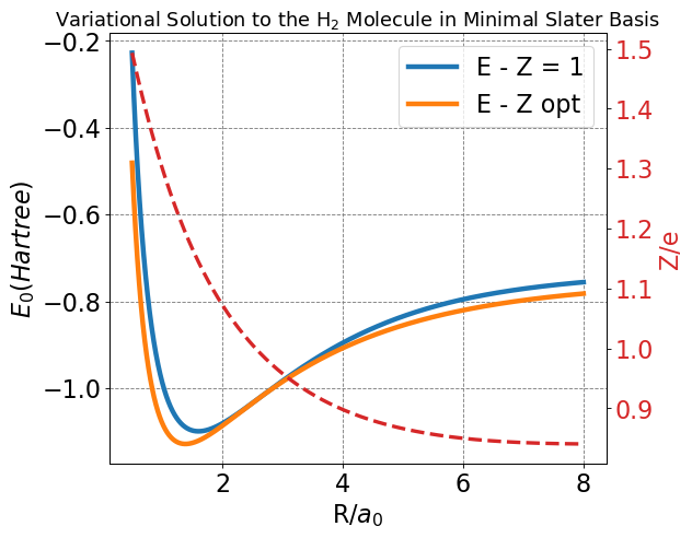
Below I will compute the energy as a function of \(R\) both for the \(Z=1\) basis as well as performing a varitiational optimization of the energy with respect to \(Z\) at each value of \(R\).
Show code cell source
# H2 MO Minimal Basis
from scipy.optimize import minimize
from scipy import integrate
import matplotlib.pyplot as plt
%matplotlib inline
import numpy as np

gamma = 0.57721

def J(R):
    return np.exp(-2*R)*(1+1/R) - 1/R
def K(R):
    return -np.exp(-R)*(1+R)
def S(R):
    return np.exp(-R)*(1 + R + R*R/3)
def S2(R):
    return np.exp(R)*(1 - R + R*R/3)
def E1_integrand(t):
    return np.exp(-t)/t
def E1(x):
    return integrate.quad(E1_integrand,x,np.infty)[0]
def J2(R):
    return 1/R - np.exp(-2*R) * (1/R + 11/8 + 0.75*R + R*R/6)
def L(R):
    return np.exp(-R) * (R + 1/8 + 5/(16*R)) + np.exp(-3*R)*(-1/8 - 5/(16*R))
def K2(R):
    term_1 = -0.2 * np.exp(-2*R) * (-25/8 + 23*R/4 + 3*R*R + R**3/3)
    term_2 = 1.2/R * (S(R)**2 * (gamma + np.log(R)) - S2(R)**2 * E1(4*R) + 2*S(R) * S2(R) * E1(2*R))
    return term_1+term_2

def E(Z,R):
    w = Z*R
    denom = 1+S(w)
    prefactor = Z/denom
    t1 = Z*(1-S(w)-2*K(w))
    t2 = -2 + 2*J(w) + 4*K(w)
    t3 = (5/16 + 0.5*J2(w) + K2(w) + 2*L(w))/denom
    return prefactor*(t1+t2+t3) + 1/R
# compute energy as function of R
R = np.arange(0.5,8,0.001)
E_1s_basis = np.empty(R.size)
E_slater_basis = np.empty(R.size)
Z_min = np.empty(R.size)
for i, r in enumerate(R):
    E_1s_basis[i] = E(1,r)
    Z_min[i] = minimize(E,1.0,args=(r)).x[0]
    E_slater_basis[i] = E(Z_min[i],r)
---------------------------------------------------------------------------
ModuleNotFoundError                       Traceback (most recent call last)
Cell In[1], line 2
      1 # H2 MO Minimal Basis
----> 2 from scipy.optimize import minimize
      3 from scipy import integrate
      4 import matplotlib.pyplot as plt

ModuleNotFoundError: No module named 'scipy'
Show code cell source
R = np.arange(0.5,8,0.001)
fig, ax = plt.subplots(figsize=(8,6),dpi= 80, facecolor='w', edgecolor='k')
plt.tick_params(axis='both',labelsize=20)
plt.grid( which='major', axis='both', color='#808080', linestyle='--')
ax.plot(R,E_1s_basis,lw=4, label=r'E - Z = 1')
ax.plot(R,E_slater_basis,lw=4, label=r'E - Z opt')
ax.set_xlabel(r'R/$a_0$',fontsize=20)
ax.set_ylabel(r'$E_0 (Hartree)$',fontsize=20)
plt.legend(fontsize=20)
ax2 = ax.twinx()
color = 'tab:red'
ax2.set_ylabel('Z/e', color=color, fontsize=20)  # we already handled the x-label with ax1
ax2.plot(R, Z_min, '--', lw=3, color=color)
ax2.tick_params(axis='y', labelcolor=color,labelsize=20)
fig.tight_layout()
plt.title(r'Variational Solution to the H$_2$ Molecule in Minimal Slater Basis',fontsize=16);
Show code cell source
min_index = np.argmin(E_1s_basis)
print("Bonding energy (Z=1):", np.round(E_1s_basis[min_index],5), "Hartree")
print("Bonding distance (Z=1):", np.round(R[min_index],5), "Bohr")
min_index = np.argmin(E_slater_basis)
print("Bonding energy (Z=opt):", np.round(E_slater_basis[min_index],5), "Hartree")
print("Bonding distance (Z=opt):", np.round(R[min_index],5), "Bohr")
print("Z at bond distance:", np.round(Z_min[min_index],5), "e")
print("Opt energy deviation (kcal/mol):",np.round((E_slater_basis[min_index]+1.174)*627.5895,2))
Bonding energy (Z=1): -1.09908 Hartree
Bonding distance (Z=1): 1.603 Bohr
Bonding energy (Z=opt): -1.12823 Hartree
Bonding distance (Z=opt): 1.385 Bohr
Z at bond distance: 1.19313 e
Opt energy deviation (kcal/mol): 28.72
4.5.20.8. Summary of Variational Solution in Minimal Basis#
We see from above that the minimal basis with \(Z=1\) yields the following
If we compare this to the experimental numbers, we see poor agreement. The bond distance is off by 0.2 Bohr, for example.
Looking at the variationally optimized energy in this basis \(Z=opt\) we find
These are significantly closer to the experimental values of -1.174 and 1.401, respectively. That said, the energy is still off by 28.72 kcal/mol.
4.5.20.9. Where/Why MO Theory (and Hartree-Fock) Fails#
We could go to the effort of improving the basis set to get better energy and bond distances but one thing we have yet to discuss is the issue with dissociation in the MO picture (this problem also exists in restrictred Hartree-Fock).
We know that the energy at dissociation should be -1 Hartree because the lowest energy state should be two ground state hydrogen atoms (infinitely separated from each other). Each of these has an energy of -0.5 Hartree and thus the total energy of -1 Hartree.
Neither of our LCAO-MO solutions achieve this dissociation limit. Indeed they continue to increase in energy even out to \(R=8\) Bohr. Additionally, in the variationally optimized solution, we see that the variational parameter, \(Z\), achieves a value below \(Z=1\) as \(R\rightarrow\infty\) even though we know that it should be going to \(Z=1\).
The problem is that the single determinant minimal basis wave function cannot capture the correct dissociation behavior. Let’s look at the wave function a bit more closely to see why
The first two terms (\(1s_A(1)1s_B(2)\) and \(1s_A(2)1s_B(1)\)) represent two hydrogen atoms each with an electron. Two terms are required to account for the indistinguishability of the electrons: there is no way of knowing which electron is sitting on which nucleus. The last two terms (\(1s_A(1)1s_A(2)\) and \(1s_B(1)1s_B(2)\)) represent functions with two electrons sitting on the same nucleus. Thus, at infinite separation, these represent a situation with an H\(^-\) ion and an H\(^+\) ion. The simple MO picture requires that these be present and that they have equal weight to the properly dissociated hydrogen atoms.
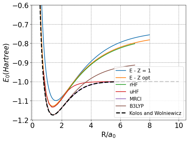
There are methods, however, that are able to predict accurate energies and dissociation behavior. Below is a plot of the energy of the H\(_2\) as a function of \(R\) for various methods (including the two we did above).
From these, we see that our two MO methods, rHF (which stands for restricted Hartree-Fock), and B3LYP (a density functional theory method) all get the incorrect dissociation behavior. uHF (unrestricted Hartree-Fock) gets the correct dissociation behavior but doesn’t do a great job getting the minimum energy correct. MRCI, or multi-reference configuation interaction, gets both right and is a very accurate method in general. We will discuss this method more.
It should be noted the B3LYP gets the position and energetics of the minimum quite well. This is generally true for DFT methods - they have been parameterized to get the minimum energy structures correct and can do so for many structures reasonably well. We will not discuss these methods any further.
Show code cell source
import numpy as np
import matplotlib.pyplot as plt
%matplotlib inline
R = np.arange(0.5,8,0.001)
fig, ax = plt.subplots(figsize=(8,6),dpi= 80, facecolor='w', edgecolor='k')
plt.tick_params(axis='both',labelsize=20)
plt.grid( which='major', axis='both', color='#808080', linestyle='--')
ax.plot(R,E_1s_basis,lw=2, label=r'E - Z = 1')
ax.plot(R,E_slater_basis,lw=2, label=r'E - Z opt')
ax.set_xlabel(r'R/$a_0$',fontsize=20)
ax.set_ylabel(r'$E_0 (Hartree)$',fontsize=20)
h2_all = np.loadtxt("h2_various_methods.txt",skiprows=1)
ax.plot(h2_all[:,0]*1.88973,h2_all[:,1],lw=2,label='rHF')
ax.plot(h2_all[:,0]*1.88973,h2_all[:,2],lw=2,label='uHF')
ax.plot(h2_all[:,0]*1.88973,h2_all[:,6],lw=2,label='MRCI')
ax.plot(h2_all[:,0]*1.88973,h2_all[:,7],lw=2,label='B3LYP')
exact = np.loadtxt("h2_kolos_wolniewicz.txt",skiprows=1)
ax.plot(exact[:,0],exact[:,1],'--',lw=3,c='k',label="Kolos and Wolniewicz")
ax.set_ylim(-1.2,-0.6)
ax.legend(fontsize=14);