4.5.13. The Hydrogen Atom Absorption Spectrum#
4.5.13.1. Motivation:#
Here we will consider the allowed absorption and emission lines of the model of the hydrogen atom stemming from the Schrodinger equation. We will also determine the selection rules for absorption/emission.
4.5.13.2. Learning Goals:#
After working through these notes, you will be able to:
Compute absorption and emission energies for the hydrogen atom.
Identify the selection rules for electronic transitions in the hydrogen atom.
4.5.13.3. Coding Concepts:#
The following coding concepts are used in this notebook:
4.5.13.4. The Hydrogen Atom Spectrum#
The allowed energies of the hydrogen atom are
An electron can be excited from one state to a higher state when the atom absorbs light of the correct frequency/energy. The allowed frequencies/energies are dictated by the energy spacings, or differences in energies.
For example, if we consider the \(n=1\) as the ground state, then the allowed energies are
This series of lines is called the Lyman series.
If we consider the \(n=2\) as the ground state, then the allowed energies are
This series of lines is called the Balmer series.
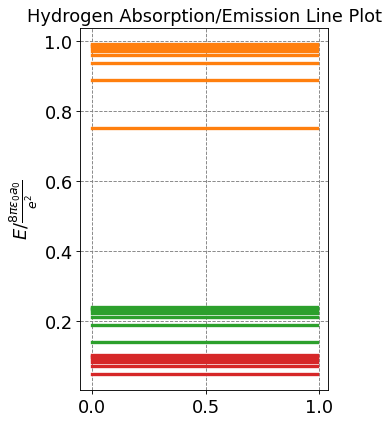
Any state can be considered as the ground state and will result in a series of absoprtion lines. Below is a plot of the lines stemming from the first three states.
Show code cell source
# let's plot some radial wavefunctions of the hydrogen atom
import matplotlib.pyplot as plt
%matplotlib inline
import numpy as np

fontsize = 16
plt.figure(figsize=(4,6),dpi= 80, facecolor='w', edgecolor='k')
plt.tick_params(axis='both',labelsize=fontsize)
plt.grid(which='major', axis='both', color='#808080', linestyle='--')
plt.title("Hydrogen Absorption/Emission Line Plot",fontsize=fontsize)
plt.ylabel(r'$E / \frac{8\pi\epsilon_0a_0}{e^2}$',size=fontsize)

# parameters for plotting
nLimit = 10

x = np.arange(0,1,0.01)
for n1 in range(1,4):
    for n2 in range(n1+1,nLimit+1):
        color = "C"+str(n1)
        En = 1/n1**2-1/n2**2
        plt.plot(x,np.ones(x.size)*En, lw=3,c=color)
#plt.legend(fontsize=12)
plt.show();
Here we have presumed that all changes in \(n\) are allowed. Below we will show that this is true but that there are selection rules for the changes in \(l\) and \(m\) that we need to consider.
4.5.13.5. The Quantum Mechanics of Spectroscopy#
Various properties of molecules and materials are probed by shining light on the system. The measurement of absorption or emission from this process is called spectroscopy. In order to discern what happens to the system when perturbed by this light, we must start by describing the light and ultimately the system dependent operator that allows the system to interact with the light.
Light produces a time dependent electromagnetic field, \(\mathbf{E}\), which can be approximatly written as
\(\mathbf{E} = \mathbf{E}_0 cos2\pi\nu t\),
where \(\nu\) is the frequency of the radiation and \(\mathbf{E}_0\) is the electric field vector. Note that this field is for monochromatic light and has an explicit time dependence.
The electromagnetic field of the light interacts with the dipole of the system. Strictly speaking, the interaction of the light with the dipole of the system affects the energy of the system and thus the Hamiltonian that one must consider when solving the Schrodinger equation. That is, the wavefunction of the molecule is perturbed by the presence of the electromagnetic field. The perturbation to the Hamiltonian can be written as
\(\hat{H}^{(1)} = -\mathbf{\mu}\cdot\mathbf{E} = -\mathbf{\mu}\cdot\mathbf{E}_0 cos2\pi\nu t\)
where \(\mathbf{\mu}\) is the dipole vector of the molecule. The complete Hamiltonian for the system is then
\(\hat{H} = \hat{H}^{(0)} + \hat{H}^{(1)}\),
where \(\hat{H}^{(0)}\) is the Hamiltonian of the isolated system. This Hamiltonian has explicit time dependence so we cannot solve the stationary state Schrodinger equation. This problem can be solved using time-dependent perturbation theory but we will not do so now. Instead we will use some of the results from this solution.
4.5.13.5.1. Transition Dipole Moment#
Time-dependent perturbation theory on the above Hamiltonian leads to defining what is called the transition dipole moment for a molecule. This is defined as
\(\langle \psi_{nlm} | \mathbf{\mu} | \psi_{n'l'm'}\rangle = \int_{-\infty}^{\infty} \psi^*_{nlm}\mathbf{\mu}\psi_{n'l'm'}dV\),
where \(\psi_{nlm}\) are stationary state solutions of the \(\hat{H}^{(0)}\) Hamiltonian of the Hydrogen atom. This quantity dictates the absorpition of a transition from state \(nlm\) to a state \(n'l'm'\). If this quantity is zero then the transition is not allowed, if the quantity is finite, the transition is allowed. This will dictate the selection rules.
To determine this quantity, we start by expresing the dipole vector as a sum of it \(x\), \(y\), and \(x\) contributions:
where \(\mathbf{i}\), \(\mathbf{j}\), \(\mathbf{k}\) are unit vectors in the \(x\), \(y\), and \(z\) directions respectively and \(\mu_x = \mathbf{\mu}\cdot\mathbf{i}\), \(\mu_y = \mathbf{\mu}\cdot\mathbf{j}\), and \(\mu_z = \mathbf{\mu}\cdot\mathbf{k}\) are the components of the dipole vector in those directions.
Thus, our transition dipole moment can now be expressed as a sum of three terms
\(\langle \psi_{nlm} | \mathbf{\mu} | \psi_{n'l'm'}\rangle = \langle \psi_{nlm} | \mu_x | \psi_{n'l'm'}\rangle\mathbf{i} + \langle \psi_{nlm} | \mu_y | \psi_{n'l'm'}\rangle\mathbf{j} + \langle \psi_{nlm} | \mu_x | \psi_{n'l'm'}\rangle\mathbf{k}\)
We now express each of the dipole moment components as a Taylor series expansion truncated at first order analagous to
\(\mu_x = \mu_{0x} + \left( \frac{d\mu_x}{dx}\right)_0x + ...\)
where \(\mu_{0x} \) is the dipole moment component at the equilibrium position and \(x\) is the displacement from that position. Substituting this expansion truncated to second order into the component of the transition dipole moment we get
\(\langle nlm | \mu_x | n'l'm'\rangle = \mu_{0x} \langle nlm | n'l'm'\rangle + \left( \frac{d\mu_x}{dx}\right)_0 \langle nlm |x| n'l'm'\rangle \).
Doing a similar procedure for the other two components yields
The first terms in these, the ones that look like \(\mu_{0x} \langle nlm | n'l'm'\rangle\), will be zero if any of the quatum number are different due to the orthogonality of the unperturbed Hydrogen atom wave functions. Thus, these are uninteresting in terms of absorption or emission becuase the are only finite for no change in state and thus no change in energy. It is the second term in each that we must evaluate to determine the selection rules.
Since we have determined the Hydrogen atom wave functions in spherical polar coordinates, we will need to convert the \(x\), \(y\), and \(x\) operators to polar coordinates to assess the selection rules. Namely, we will determine the following expectation values to determine the selection rules
4.5.13.5.2. No selection rules for \(r\) and \(n\)#
The \(r\) dependent terms of the transition dipole moment can be all boiled down to the form
It turns out that these are all finite meaning that there are no limitations on what \(n'\) or \(l'\) values can be taken based on the radial component of the wave function.
Rather than deriving this I show it by numeric integration for a select subset of possible transitions. We see below that all of these expectation values are finite. The real implication for this is that transitions are allowed between any primary quantum numbers of the hydrogen atom.
Show code cell source
import numpy as np
from scipy import integrate
from scipy.special import eval_genlaguerre
from scipy.special import factorial
a0 = 1.0 # radial unit of Bohr!
def hydrogen_atom_radial_wf(r,n,l):
    R_prefactor = -np.sqrt(factorial(n-l-1)/(2*n*factorial(n+l)))*(2.0/(n*a0))**(l+1.5)*np.power(r,l)*np.exp(-r/(n*a0))
    return R_prefactor*eval_genlaguerre(n-l-1,2*l+1,2*r/(n*a0))
def integrand(r,n1,l1,n2,l2):
    return r*r*r*hydrogen_atom_radial_wf(r,n1,l1)*hydrogen_atom_radial_wf(r,n2,l2)

print ("{:<10} {:<10} {:<10} {:<10} {:<20}".format('n', 'l', 'n\'', 'l\'', '<R_nl | r | R_n\'l\'>'))
print("--------------------------------------------------------------------")
for n1 in range(1,4):
    for l1 in range(n1):
        for n2 in range(1,4):
            for l2 in range(n2):
                print ("{:<10} {:<10} {:<10} {:<10} {:<20}".format(n1, l1, n2, l2, np.round(integrate.quad(integrand,0,np.infty,args=(n1,l1,n2,l2))[0],3)))
n          l          n'         l'         <R_nl | r | R_n'l'>
--------------------------------------------------------------------
1          0          1          0          1.5
1          0          2          0          -0.559
1          0          2          1          1.29
1          0          3          0          -0.244
1          0          3          1          0.517
1          0          3          2          0.385
2          0          1          0          -0.559
2          0          2          0          6.0
2          0          2          1          -5.196
2          0          3          0          -1.851
2          0          3          1          3.065
2          0          3          2          -5.939
2          1          1          0          1.29
2          1          2          0          -5.196
2          1          2          1          5.0
2          1          3          0          0.938
2          1          3          1          -1.769
2          1          3          2          4.748
3          0          1          0          -0.244
3          0          2          0          -1.851
3          0          2          1          0.938
3          0          3          0          13.5
3          0          3          1          -12.728
3          0          3          2          9.487
3          1          1          0          0.517
3          1          2          0          3.065
3          1          2          1          -1.769
3          1          3          0          -12.728
3          1          3          1          12.5
3          1          3          2          -10.062
3          2          1          0          0.385
3          2          2          0          -5.939
3          2          2          1          4.748
3          2          3          0          9.487
3          2          3          1          -10.062
3          2          3          2          10.5
4.5.13.5.3. Selection rule for \(l\) and \(m\) from \(\theta\) and \(\phi\)#
The \(\theta\) and \(\phi\) dependent terms of the transition dipole moment are
We will evaluate these terms using numeric integration:
Show code cell source
from scipy import integrate
from scipy.special import lpmv
import numpy as np
from scipy.special import factorial

def theta_norm(m,l):
    return np.sqrt(((2*l+1)*factorial(l-np.abs(m)))/(2*factorial(l+np.abs(m))))
def cos_integrand(theta,l1,m1,l2,m2):
    return theta*theta_norm(m1,l1)*theta_norm(m2,l2)*lpmv(m1,l1,theta)*lpmv(m2,l2,theta)
def sin_integrand(theta,l1,m1,l2,m2):
    return np.sin(theta)**2*theta_norm(m1,l1)*theta_norm(m2,l2)*lpmv(m1,l1,np.cos(theta))*lpmv(m2,l2,np.cos(theta))
def phi_norm2():
    return 1/(2*np.pi)
def phi_cos_integrand(phi,m1,m2):
    real_part = phi_norm2()*(np.cos(m1*phi)*np.cos(m2*phi)+np.sin(m1*phi)*np.sin(m2*phi))
    return np.cos(phi)*real_part
def phi_sin_integrand(phi,m1,m2):
    real_part = phi_norm2()*(np.cos(m1*phi)*np.cos(m2*phi)+np.sin(m1*phi)*np.sin(m2*phi))
    return np.cos(phi)*real_part
def phi_integrand(phi,m1,m2):
    real_part = phi_norm2()*(np.cos(m1*phi)*np.cos(m2*phi)+np.sin(m1*phi)*np.sin(m2*phi))
    return real_part


print ("{:<8} {:<8} {:<35} {:<35} {:<35}".format('∆l','∆m','<Y_lm|sin_theta cos_phi|Y_l\'m\'>', '<Y_lm|sin_theta sin_phi|Y_l\'m\'>','<Y_lm|cos_theta|Y_l\'m\'>'))
print("------------------------------------------------------------------------------------------------------")
for l1 in range(3):
    for m1 in range(l1+1):
        for l2 in range(3):
            for m2 in range(l2+1):
                sin_theta_cos_phi = integrate.quad(sin_integrand,0,np.pi,args=(l1,m1,l2,m2))[0]*integrate.quad(phi_cos_integrand,0,2*np.pi,args=(m1,m2))[0]
                sin_theta_sin_phi = integrate.quad(sin_integrand,0,np.pi,args=(l1,m1,l2,m2))[0]*integrate.quad(phi_sin_integrand,0,2*np.pi,args=(m1,m2))[0]
                cos_theta = integrate.quad(cos_integrand,-1,1,args=(l1,m1,l2,m2))[0]*integrate.quad(phi_integrand,0,2*np.pi,args=(m1,m2))[0]
                print ("{:<8} {:<8} {:<35} {:<35} {:<35}".format(l1-l2,m1-m2,np.round(sin_theta_cos_phi,3),np.round(sin_theta_sin_phi,3),np.round(cos_theta,3)))
∆l       ∆m       <Y_lm|sin_theta cos_phi|Y_l'm'>     <Y_lm|sin_theta sin_phi|Y_l'm'>     <Y_lm|cos_theta|Y_l'm'>
------------------------------------------------------------------------------------------------------
0        0        0.0                                 0.0                                 0.0
-1       0        0.0                                 0.0                                 0.577
-1       -1       -0.408                              -0.408                              0.0
-2       0        -0.0                                -0.0                                0.0
-2       -1       -0.0                                -0.0                                -0.0
-2       -2       -0.0                                -0.0                                -0.0
1        0        0.0                                 0.0                                 0.577
0        0        0.0                                 0.0                                 0.0
0        -1       -0.0                                -0.0                                -0.0
-1       0        0.0                                 0.0                                 0.516
-1       -1       -0.316                              -0.316                              -0.0
-1       -2       -0.0                                -0.0                                -0.0
1        1        -0.408                              -0.408                              0.0
0        1        -0.0                                -0.0                                -0.0
0        0        0.0                                 0.0                                 0.0
-1       1        0.183                               0.183                               -0.0
-1       0        0.0                                 0.0                                 0.447
-1       -1       -0.447                              -0.447                              0.0
2        0        -0.0                                -0.0                                0.0
1        0        0.0                                 0.0                                 0.516
1        -1       0.183                               0.183                               -0.0
0        0        0.0                                 0.0                                 0.0
0        -1       -0.0                                -0.0                                -0.0
0        -2       0.0                                 0.0                                 -0.0
2        1        -0.0                                -0.0                                -0.0
1        1        -0.316                              -0.316                              -0.0
1        0        0.0                                 0.0                                 0.447
0        1        -0.0                                -0.0                                -0.0
0        0        0.0                                 0.0                                 0.0
0        -1       -0.0                                -0.0                                -0.0
2        2        -0.0                                -0.0                                -0.0
1        2        -0.0                                -0.0                                -0.0
1        1        -0.447                              -0.447                              0.0
0        2        0.0                                 0.0                                 -0.0
0        1        -0.0                                -0.0                                -0.0
0        0        0.0                                 0.0                                 0.0
We see that there are finite values for at least one of the expectation values when
These are the selection rules of the hydrogen atom.
4.5.13.6. Summary of Selection Rules for the Hydrogen Atom#
A transition from any primary quantum number to any other primary quantum number is allowed. But, a transition requires a change in the angular momentum quantum number \(l\). This implies that the \(1s \rightarrow 2s\) transition is forbidden.