4.2.7. Kinetic Theory of Gasses from the Classical Ideal Gas

4.2.7.1. Motivation

In these notes we will demonstrate that some of the aspects of the Kinetic Theory of Gasses can be derived from the partition function of the classical ideal gas.

4.2.7.2. Learning Goals

After these notes, students should be able to:

1. Derive the relationship between average squared particle speed and temperature for a gas.

2. Derive the Gaussian distribution of components of a particle velocity

3. Derive the distribution of speeds for a gas from the classical partition function.

4.2.7.3. Coding Concepts

1. variables

2. functions

3. plotting with matplotlib

4.2.7.4. Introduction

The Kinetic Theory of Gasses (KTG) is a model of Gasses that is used to explain attributes of all gasses including:

1. The relationship between temperature and average particle velocity

2. Components of the velocity of a gas follow a Gaussian distribution (constant V and T)

3. The speed of a gas follow a Maxwell-Boltzmann distribution

The KTG is used to describe other attributes of a gas that we will not discuss here, including some that cannot be derived from an ideal gas.

The three attributes above can be derived from the partition function of a classical ideal gas.

Recall that the partition function for a classical ideal gas

(4.161)\[\begin{equation} Q = \frac{V^N\left( \frac{2\pi mk_BT}{h^2}\right)^{3N/2}}{N!} \end{equation}\]

and that this was derived by representing the energy of the system as:

(4.162)\[\begin{equation} H(\vec{R}^N,\vec{P}^N) = \sum_{i=1}^N \frac{\vec{p}_i^2}{2m} \end{equation}\]

We derived this by utilizing an integral overall all phase space (phase space is composed of position and momenta)

(4.163)\[\begin{equation} Q = \frac{\int_0^L\int_{-\infty}^{\infty} e^{-\beta H(\vec{R}^N,\vec{P}^N)}d\vec{R}^Nd\vec{P}^N}{h^{3N}N!} \end{equation}\]

4.2.7.5. Temperature is related to average squared velocity for a gas

To demonstrate the relationship between average squared particle velocity and temperature we will compute the average energy of a classical ideal gas

(4.164)\[\begin{eqnarray} \langle E \rangle &=& \langle H(\vec{R}^N,\vec{P}^N) \rangle \\ &=& \langle \sum_{i=1}^N \frac{\vec{p}_i^2}{2m} \rangle \\ &=& \frac{1}{2m} \sum_{i=1}^N \langle \vec{p}_i^2 \rangle \\ &=& \frac{1}{2m} N \langle \vec{p}^2 \rangle \end{eqnarray}\]

where the last equality holds because all particles are equivalent and thus \(\langle \vec{p}_i^2 \rangle = \langle \vec{p}_j^2 \rangle\) for all \(i\) and \(j\).

Next we recognize that \(\vec{p} = m\vec{v}\) to get

(4.165)\[\begin{eqnarray} \langle E \rangle &=& \frac{1}{2m} N m^2 \langle \vec{v}^2 \rangle \\ &=& \frac{Nm}{2} \langle \vec{v}^2 \rangle \end{eqnarray}\]

To determine the relationship with temperature recall that

(4.166)\[\begin{equation} \langle E \rangle = -\left( \frac{\partial \ln Q}{\partial \beta}\right) \end{equation}\]

where

(4.167)\[\begin{eqnarray} lnQ = -\frac{3N}{2}\ln \beta + \frac{3N}{2}\ln\left( \frac{2\pi m}{h^2}\right) \ln V - \ln N! \end{eqnarray}\]

Differentiating w.r.t. \(\beta\)

(4.168)\[\begin{equation} \langle E \rangle = \frac{3Nk_BT}{2} \end{equation}\]

Equating the two expressions for \(\langle E \rangle\) yields

(4.169)\[\begin{eqnarray} \frac{3Nk_BT}{2} &=& \frac{Nm}{2} \langle \vec{v}^2 \rangle \\ \Rightarrow T &=& \frac{m}{3k_B} \langle \vec{v}^2 \rangle \end{eqnarray}\]

In molar quantities this becomes

(4.170)\[\begin{eqnarray} T = \frac{M}{3R} \langle \vec{v}^2 \rangle \end{eqnarray}\]

or

(4.171)\[\begin{eqnarray} \frac{3RT}{M} = \langle \vec{v}^2 \rangle \end{eqnarray}\]

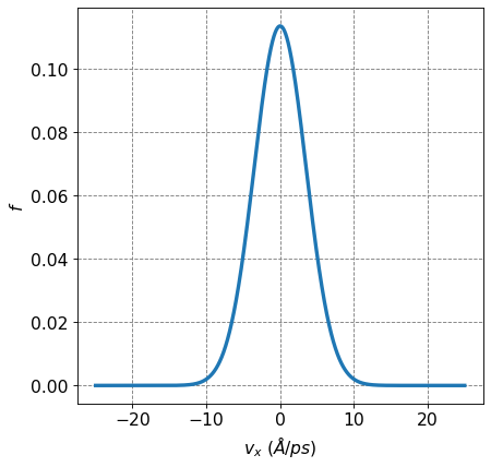
4.2.7.6. Distribution of Components of Particle Velocity Follow a Gaussian

We have seen this equation before but the KTG states that components of particle velocity, \(\vec{v} = (v_x,v_y,v_z)\), follow a Gaussian distribution of the form

(4.172)\[\begin{equation} f(v_x) = \left( \frac{M}{2\pi RT}\right)^{1/2}e^{-\frac{Mv_x^2}{2RT}} \end{equation}\]

where \(M\) is the molar of the particles. The other components, \(v_y\) and \(v_z\), have analagous distributions \(f(v_y)\) and \(f(v_z)\).

We are going to derive this equation from the partition function and Boltzmann factors from a classical monatomic ideal gas.

From standard classical statistical mechanics we recall that the probability of a state described by continuous variable \(x\) is given as

(4.173)\[\begin{equation} P(x) = \frac{e^{-\beta E(x)}}{Q} \end{equation}\]

In the case of particle velocities component \(v_x\) for a classical monatomic ideal gas we consider

(4.174)\[\begin{eqnarray} P(v_x) = \frac{e^{-\beta H_{1D}(v_x)}}{q_{1D}} \end{eqnarray}\]

where H_{1D} is the Hamiltonian that only depends on the single velocity component and \(q_{1D}\) is the partition function in 1D of velocties. This can also be determined by using the total \(q\) and including a degeneracy for \(e^{-\beta H_{1D}(v_x)}\) that involves and integration over positions and two of the orthogonal velocity dimensions. The results will be the same.

We get

(4.175)\[\begin{eqnarray} P(v_x) &=& \frac{e^{-\beta H_{1D}(v_x)}}{Q_{1D}} \\ &=& \frac{e^{-\beta \frac{1}{2}mv_x^2}}{\left( \frac{2\pi mk_BT}{h^2}\right)^{1/2}} \\ &=& \left( \frac{h^2}{2\pi mk_BT}\right)^{1/2}e^{-\beta \frac{1}{2}mv_x^2} \\ &=& \left( \frac{h^2}{2\pi MRT}\right)^{1/2}e^{- \frac{1}{RT}Mv_x^2}, \end{eqnarray}\]

where the last step we convert to molar quantities.

Compare this equation for \(P(v_x)\) to the KMT equation \(f(v_x)\) above we see some differences. Namely they differ by a factor of \(\frac{M}{h}\)

# plot Gaussian distribution of Ne velocity component at T=300
import numpy as np
import matplotlib.pyplot as plt
m = 20.180   #amu
kB = 1.380649e4/1.66  # m2 amu s-2 K-1
kB *= 1e-4  # Ang^2 amu ps-2 K-1
T = 300 # K
def f(vx):
    return np.sqrt(m/(2*np.pi*kB*T)) * np.exp(-m*vx**2/(2*kB*T))
fontsize=14
vx = np.arange(-25,25,0.01)
fig = plt.figure(figsize=(6,6), dpi= 80, facecolor='w', edgecolor='k')
ax = plt.subplot(111)
ax.grid(b=True, which='major', axis='both', color='#808080', linestyle='--')
ax.set_xlabel("$v_x$ $(\AA/ps)$",size=fontsize)
ax.set_ylabel("$f$",size=fontsize)
plt.tick_params(axis='both',labelsize=fontsize)
plt.plot(vx,f(vx),lw=3)

[<matplotlib.lines.Line2D at 0x7fd3de9174f0>]

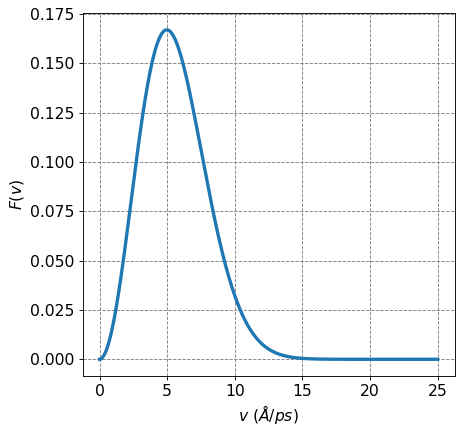
4.2.7.7. Distribution of Particle Speed is the Maxwell-Boltzmann Distribution

The distribution of particle speed is termed the Maxwell-Boltzmann distribution and has the following for

(4.176)\[\begin{equation} F(v) = 4\pi\left(\frac{m}{2\pi k_BT}\right)^{3/2}v^2e^{-mv^2/2k_B T} \end{equation}\]

To derive this expression, we use a similar procedure to above except in this case we pay attention to the degeneracy of a particular value of \(v\):

(4.177)\[\begin{equation} P(v) = \frac{g_ve^{-\beta H(v)}}{Q}. \end{equation}\]

The degeneracy of a particular value of \(v\) is \(g_v=4\pi v^2\), this can be demonstrated in a variety of ways but here I will just give a qualitative argument. A particular value for \(v=\sqrt{v_x^2+v_y^2+v_z^2}\) can be achieved with various values of \(v_x\), \(v_y\), and \(v_z\). The size of the degeneracy increases as the value of \(v\) increases. More specifically, a value for \(v\) carves out the surface of a sphere hence the degeneracty of \(4\pi v^2\).

Given this, we now have

(4.178)\[\begin{eqnarray} P(v) &=& \frac{4\pi v^2e^{-\beta \frac{1}{2}mv^2}}{\left(\frac{2\pi mk_BT}{h^2}\right)^{3/2}} \\ &=& 4\pi\left(\frac{h^2}{2\pi mk_BT}\right)^{3/2} v^2e^{-\frac{mv^2}{2k_BT}} \end{eqnarray}\]

Compare this equation for \(P(v)\) to the KMT equation \(F(v)\) above we see some differences. Namely they differ by a factor of \(\frac{m^3}{h^3}\) or a factor of \(\frac{m}{h}\) in each direction.

# plot Gaussian distribution of Ne velocity component at T=300
import numpy as np
import matplotlib.pyplot as plt
m = 20.180   #amu
kB = 1.380649e4/1.66  # m2 amu s-2 K-1
kB *= 1e-4  # Ang^2 amu ps-2 K-1
T = 300 # K
def F(v):
    return 4*np.pi*np.sqrt(m/(2*np.pi*kB*T))**3 * v**2* np.exp(-m*v**2/(2*kB*T))
fontsize=14
v = np.arange(0,25,0.01)
fig = plt.figure(figsize=(6,6), dpi= 80, facecolor='w', edgecolor='k')
ax = plt.subplot(111)
ax.grid(b=True, which='major', axis='both', color='#808080', linestyle='--')
ax.set_xlabel("$v$ $(\AA/ps)$",size=fontsize)
ax.set_ylabel("$F(v)$",size=fontsize)
plt.tick_params(axis='both',labelsize=fontsize)
plt.plot(v,F(v),lw=3)

[<matplotlib.lines.Line2D at 0x7fd3dead7880>]