4.5.3. Schrodinger Equation#
4.5.3.1. Motivation#
The Schrodinger equation is the fundamental equation of quantum mechanics. In these notes, we introduce the Schrodinger equation and its relationship to the classical wave equation. Motivated by the Hamiltonian operator in the Schrodinger equation, we then introduce the concept of operators in quantum mechanics.
4.5.3.2. Learning Goals#
After working through these notes, you will be able to:
Write out and identify the Schrodinger equation
Demonstrate the equivalence of the Schrodinger equation and the classical wave equation
Define an opertor
Apply operators to functions
Define a linear operator
Identify linear operators
4.5.3.3. Coding Concepts#
No coding concepts are used. Yet.
4.5.3.4. Schrodinger Equation from the Classical Wave Equation#
The Schrodinger equation is the basis for all of the quantum mechanics we will discuss in this class. Specifically, the time independent Schrodinger equation is all we will discuss in this class. This equation has the well known form
where \(\bar{H}\) is the Hamiltonian operator, \(\Psi\) is the wave function, and \(E\) is the energy. This equation cannot be derived from any more basic equations, rather we have to accept the Schrodinger equations as one of the postulates of quantum mechanics.
The classical wave equation can be manipulated into a Schrodinger equation. To see this, recall that the classical wave equation can be written as
for solution
Now recall that \(\omega = 2\pi\nu\) and \(v = \nu\lambda\) meaning we can write the differential equation as
Now recall from the de Broglie wave equation that we can write
where the last equality holds because \(E = K + V = \frac{1}{2}mv^2 + V\). Plugging this relationship in for \(\lambda\) in the classical wave equation we get
We see that this looks like the Schrodinger equation with
4.5.3.5. Operators#
We see that the Hamiltonian in the Schrodinger equation is an operator. Operators are symbols that describe performing a mathematical operation. Examples of operators include derivative with respect to \(x\), \(\frac{d}{dx}\), multiply by \(x\), simply denoted \(x\), and integrate, denoted \(\int\).
We denote generic operators by characters (often capital letters) with hats over them. For example below we define the operator \(\hat{A}\) as the first derivative with respect to \(x\):
Operators by themselves are pretty useless. The must be applied to a function. We might apply the operator \(\hat{A}\), above, a generic function of one dimension:
If we know the specific function, \(f(x) = 2x\) for example, we can determine the result of operating \(\hat{A}\) on \(f(x)\):
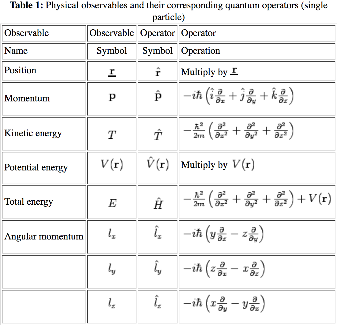
Operators are very important in quantum mechanics. Specifically, applying operators to the wavefunction for a system can be used to determine physical obervables for that system. Below is a table of classical observables and the corresponding quantum mechanical operator.
Classical and quantum correspondence.
Operators can be divided into linear operators and non-linear operators. We will focus on linear operators.
4.5.3.5.1. Example: Operators#
Perform the following operations
\(\hat{A}(2x)\), \(\hat{A} = \frac{d^2}{dx^2}\)
\(\hat{A}(x^2)\), \(\hat{A} = \frac{d^2}{dx^2} + 2\frac{d}{dx} + 3\)
\(\hat{A}(xy^3)\), \(\hat{A} = \frac{\partial}{\partial y}\)
4.5.3.5.2. Linear Operators#
A linear operator, \(\hat{A}\), has the following property:
\(\hat{A} \left[ c_1f_1(x) + c_2f_2(x)\right] = c_1\hat{A}f_1(x) + c_2\hat{A}f_2(x)\)
There are plenty of examples of linear operators including differentiation and integration. Taking the square root, however, is an example of an operator that is not linear.
In order to determine if an operator is linear, we must apply it to a sum of arbitrary functions and demonstrate that the above equality holds.
4.5.3.5.3. Example: Linear Operators#
Which of the following are linear operators?
\(\hat{A} = \frac{d}{dx}\)
\(\hat{A} = \sqrt{}\)
\(\hat{A} = \frac{\partial}{\partial y} + \frac{\partial}{\partial x}\)