4.5.6. The Postulates and Formalism of Quantum Mechanics

4.5.6.1. Postulates

Postulate 1: The state of a quantum-mechanical system is completely specified by a function \(\Psi (\mathbf{r},t)\) that depends on the coordinates of the particle and on time. This function, called the wavefunction, has the important property that \(\Psi^*(\mathbf{r},t)\Psi(\mathbf{r},t)dxdydz\) is the probability that the particle lies in the volume element \(dxdydz\) located at \(\mathbf{r}\) at time \(t\).

The above postulate is written for a single particle system. The same holds for a system of many particles. In this case we write \(\mathbf{r} = (\mathbf{r_1},\mathbf{r_1},...,\mathbf{r_N}) = ((x_1,y_1,z_1),(x_2,y_2,z_2),...,(x_N,y_N,z_N))\) for an \(N\) particle system. Note this also mean that we must integrate over each \(x_i\), \(y_i\) and \(z_i\). We abbreviate this by writing \(d\tau\) to denote integration over all degrees of freedom of all particles. So for an \(N\) particle system we can write that \(\Psi^*(\mathbf{r},t)\Psi(\mathbf{r},t)d\tau\) denotes the probability of finding the \(N\) particles in the hyper volume element \(d\tau\) located at \(\mathbf{r}\) at time t.

Wave functions are typically normalized. This means that the probability of finding the particle somewhere in the space is 1. This can be written mathematically as:

\(\int_{-\infty}^{\infty} \Psi^*(\mathbf{r},t)\Psi(\mathbf{r},t)d\tau = 1.\)

Example 4-1: Making sure wave functions are normalized.

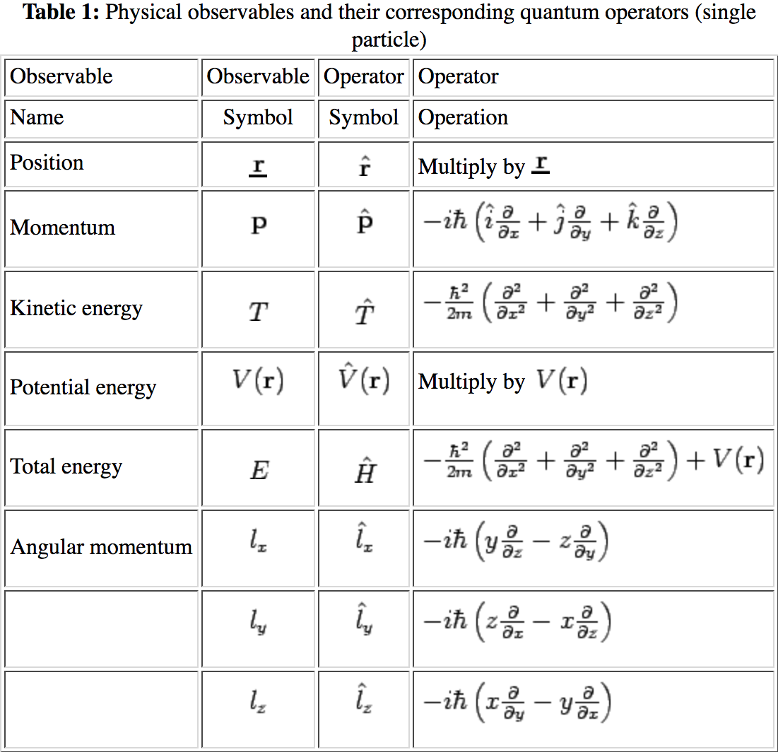
Postulate 2: To every observable in classical mechanics there corresponds a linear, Hermition operator in quantum mehcanics.

An operator is a symbol that tells you to do something to whatever follows that symbol. We have encountered numerous operators. These include differentiate by x, \(d/dx\), differentiate by y, \(d/dy\), integrate, take the sqaure root and others.

A linear operator, \(\hat{A}\), has the following property:

\(\hat{A} \left[ c_1f_1(x) + c_2f_2(x)\right] = c_1\hat{A}f_1(x) + c_2\hat{A}f_2(x)\)

There are plenty of examples of linear operators including differentiation and integration. Taking the square root, however, is an example of an operator that is not linear. Show this…

Quantum mechanical operators must be Hermitian meaning that they have real valued eigenvalues. This is, in part, a consquenece of postulate 3 but in general quantum mechanical operators lead to osbervable quantities that must be real. To determine if an operator, \(\hat{A}\), is Hermitian it must obey the following relationship:

\(\int_{\infty}^{\infty} f^*\hat{A}fdx = \int_{-\infty}^{\infty}f\hat{A}^*f^*dx\)

Example: Is the operator \(d/dx\) Hermitian?

\(\int_{-\infty}^{\infty} f^*\frac{d}{dx}fdx\)

Start by integrating by parts to get:

\( = f^*f|_{-\infty}^{\infty} - \int_{-\infty}^{\infty} f \frac{df^*}{dx} dx\)

The first term must be zero because a well-behave wave function must vanish at infinity. So now we have the left hand side of the above equation which must be equal to the right hand side from the equation defining a Hermition operator so we get:

\( - \int_{-\infty}^{\infty} f \frac{df^*}{dx} dx =? \int_{-\infty}^{\infty} f \frac{df^*}{dx}dx\)

In general this will not hold so the operator \(d/dx\) is not Hermitian.

Classical and quantum correspondence. Table 4.1 in McQuarrie.

Postulate 3: Measurement of an observable corresponding to operator \(\hat{A}\), the only values that will ever be observed are the eigenvalues \(a\), which satisfy the eigenvalue equation:

\(\hat{A}\Psi_a = a\Psi_a\)

In general there will be a set of eigenvalues, \(\{a_n\}\), corresponding to an operator \(\hat{A}\). Postulate 3 can be rewritten as

\(\hat{A}\Psi_n = a_n\Psi_n\)

Postulate 4: If a system is in a state described by a normalized wave function \(\Psi\), then the average value of the observable corresponding to \(\hat{A}\) is given by

\(\langle a \rangle = \int_{-\infty}^{\infty}\Psi^*\hat{A}\Psi d\tau\)

Example 4-4:

Suppose that a particle in a box is in the state represented by the normalized wave function:

\(\Psi(x) = \begin{cases} \left( \frac{30}{a^5}\right)^{1/2}x(a-x),& 0\leq x\leq a\\ 0,& \text{otherwise} \end{cases}\)

Calculate the average energy of the system.

SOLUTION: The problem states that \(\Psi(x)\) is normalized so we need not worry about renormalizing it. We setup the average integral as:

\(\langle E \rangle = \int_{0}^{a}\Psi^*(x)\hat{H}\Psi(x) dx = \int_0^a \Psi^*(x)\left( -\frac{\hbar^2}{2m}\frac{d^2}{dx^2}\right)\Psi(x)dx \)

Where we have put in the kinetic energy operator for the Hamiltonian. The problem states that there is a particle in a box but nothing else so we can only assume that there is kinetic energy and nothing else. Now we just need to plug in for \(\Psi(x)\) and solve the integral:

\(\langle E \rangle = \int_0^a \left( \frac{30}{a^5}\right)^{1/2}x(a-x) \left[ -\frac{\hbar^2}{2m}\frac{d^2}{dx^2}\left( \frac{30}{a^5}\right)^{1/2}x(a-x)\right] dx \)

\( = -\frac{\hbar^2}{2m}\frac{30}{a^5}\int_0^a x(a-x) \left[\frac{d^2}{dx^2} x(a-x)\right] dx \)

\( = -\frac{15\hbar^2}{ma^5}\int_0^a x(a-x) \left[\frac{d}{dx}-2x+a\right] dx \)

\( = \frac{30\hbar^2}{ma^5}\int_0^a x(a-x) dx \)

\( = \frac{30\hbar^2}{ma^5}\left[ \frac{ax^2}{2} - \frac{x^3}{3} \right]_0^a \)

\( = \frac{30\hbar^2}{ma^5}\left[ \frac{a^3}{2} - \frac{a^3}{3} \right] \)

\( = \frac{30\hbar^2}{ma^5}\left[ \frac{a^3}{6}\right] \)

\( = \frac{5\hbar^2}{ma^2} \)

4.5.6.2. Formalism

Schrodinger Equation

The Schrodinger equation is simply the application of the Hamiltonian operator to the wave function of the system. The eigenvalues of the Hamiltonian are the energy levels of the system. The Hamiltonian operator is special in the same way the energy function of a classical system is a special observable. The Schrodinger equation is commonly written as:

\(\hat{H}\Psi = E\Psi\)

It should be noted that, in general, the Schrodinger equation is time dependent. This typically shows up in the time dependence of \(\Psi(\mathbf{r},t)\). The fully time dependent Schrodinger equation is written as:

\(\hat{H}\Psi(\mathbf{r},t) = i\hbar \frac{\partial \Psi}{\partial t}\)

Where we not that \(\hat{H}\) does not explicitly depend on time (commonly the case but there are exceptions). In this case, we can perform a separation of variables on the wave function

\(\Psi(\mathbf{r},t) = \psi(\mathbf{r})f(t)\)

We can now substitue the above equation into the time dependent Schrodinger equation and divide both sides by \(\psi(\mathbf{r})\) to get:

\(\frac{1}{\psi(\mathbf{r})} \hat{H} \psi(\mathbf{r}) = \frac{i\hbar}{f(t)} \frac{df}{dt}\).

The left-hand side of this equation is time-independent and the right-hand side is position independent so they must be equal to a constant, \(E\). Thus, if the Hamiltonian of a system does not depend on time we can solve for the energy of the system using the stationary state Schrodinger equation:

\(\hat{H}\psi(\mathbf{r}) = E\psi(\mathbf{r})\).

Dirac notation

Interestingly, McQuarrie does not use Dirac notation. I think it is important for you to understand that it exists and not to get too confused by it. Here I will provide a brief set of correspondences and we may discuss more later if it comes up.

Any element of a vector space is called a ket vector. This includes wave functions. Thus we get a correspondence:

\(\psi(\mathbf{r}) \leftrightarrow |\psi\rangle\)

where the right hand side of the above relationship is the ket vector depiction of wave function \(\psi(\mathbf{r})\). To operate a linear operator, \(\hat{A}\), on the wave function we simply have:

\(\hat{A}\psi(\mathbf{r}) \leftrightarrow \hat{A}|\psi\rangle\).

To denote the complex conjugate of \(\psi(\mathbf{r})\) we use the superscript * in Schrodinger notation. In Dirac notation this is indicated as a bra vector,

\(\psi(\mathbf{r})^* \leftrightarrow \langle\psi|\).

Thus, to indicate the normalization of wave function \(\psi(\mathbf{r})\) we have:

\(\int_{-\infty}^{\infty} \psi(\mathbf{r})^*\psi(\mathbf{r}) d\tau \leftrightarrow \langle\psi|\psi\rangle = 1\).

Similarly, if we want to compute the average value of operator, \(\hat{A}\), we have:

\(\langle a \rangle = \int_{-\infty}^{\infty} \psi(\mathbf{r})^*\hat{A}\psi(\mathbf{r}) d\tau = \langle\psi|\hat{A}|\psi\rangle\).