4.5.10. Properties of Particle in a Sphere

4.5.10.1. Motivation

In our previous notes, we determined the wave functions and energies allowed for a particle inside a sphere. In these notes, we will calculate properties of a particle trapped in a sphere from these wave functions.

4.5.10.2. Learning Goals

After working through this notebook, you should be able to:

1. Normalize the particle in a sphere wavefunctions.

2. Compute the probability density of a particle in a sphere.

3. Estimate the probability of observing a particle in different regions of the sphere.

4. Compute average quantities for a particle in a sphere.

4.5.10.3. Coding Concepts

The following coding concepts are used in this notebook:

1. Variables

2. Functions

3. Plotting with matplotlib

4.5.10.4. Normalization

Before we can compute any properties of the particle in a sphere, we need to ensure that the wave functions are normalized. This means that

(4.837)\[\begin{equation} \langle \psi_{nlm}|\psi_{nlm} \rangle = 1 \end{equation}\]

Because the wave function is defined in spherical polar coordinates, this means that

(4.838)\[\begin{equation} \langle \psi_{nlm}|\psi_{nlm} \rangle = \int_0^{r_0}\int_0^{\pi}\int_0^{2\pi} \psi_{nlm}^*(r,\theta,\phi)\psi_{nlm}(r,\theta,\phi)r^2\sin\theta drd\theta d\phi= 1 \end{equation}\]

From previous notes we showed that for a particle in a sphere of radius \(r_0\)

(4.839)\[\begin{align} \psi(r,\theta,\phi) &= R_{l,n}(r)Y_l^m(\theta,\phi) \\ &= A_{nlm}j_l\left(\frac{\beta_{n,l}}{r_0}r\right)P_l^{|m|}(\cos\theta)e^{im\phi} \end{align}\]

where \(A_{nlm}\) is the normalization constant the value of which may depend on quantum numbers \(n\), \(l\), and \(m\), \(j_l(x)\) is the an \(l\)th order spherical Bessel function of the first type, \(\beta_{n,l}\) is the \(n\)th zero of the \(l\)th order spherical Bessel function of the first type, and \(P_l^{|m|}(x)\) are the associated Legendre polynomials.

We will determine the value of \(A_{nlm}\) from the normalization criterion.

(4.840)\[\begin{align} 1 &= \int_0^{r_0}\int_0^{\pi}\int_0^{2\pi} \psi_{nlm}^*(r,\theta,\phi)\psi_{nlm}(r,\theta,\phi)r^2\sin\theta drd\theta d\phi \\ &= A_{nlm}^2\int_0^{r_0}\int_0^{\pi}\int_0^{2\pi}\left(j_l\left(\frac{\beta_{n,l}}{r_0}r\right)P_l^{|m|}(\cos\theta)e^{im\phi}\right)^*j_l\left(\frac{\beta_{n,l}}{r_0}r\right)P_l^{|m|}(\cos\theta)e^{im\phi} r^2\sin\theta drd\theta d\phi \\ &= A_{nlm}^2\int_0^{r_0}\int_0^{\pi}\int_0^{2\pi} j_l\left(\frac{\beta_{n,l}}{r_0}r\right)P_l^{|m|}(\cos\theta)e^{-im\phi}j_l\left(\frac{\beta_{n,l}}{r_0}r\right)P_l^{|m|}(\cos\theta)e^{im\phi} r^2\sin\theta drd\theta d\phi \\ &= A_{nlm}^2\int_0^{r_0}\int_0^{\pi}\int_0^{2\pi}\left[j_l\left(\frac{\beta_{n,l}}{r_0}r\right)\right]^2\left[P_l^{|m|}(\cos\theta)\right]^2e^{-im\phi}e^{im\phi} r^2\sin\theta drd\theta d\phi \\ &= A_{nlm}^2\int_0^{r_0}\left[j_l\left(\frac{\beta_{n,l}}{r_0}r\right)\right]^2r^2dr \int_0^{\pi}\left[P_l^{|m|}(\cos\theta)\right]^2\sin\theta d\theta\int_0^{2\pi} d\phi \\ &= A_{r}^2\int_0^{r_0}\left[j_l\left(\frac{\beta_{n,l}}{r_0}r\right)\right]^2r^2dr\cdot A_\theta^2 \int_0^{\pi}\left[P_l^{|m|}(\cos\theta)\right]^2\sin\theta d\theta \cdot A_\phi^2\int_0^{2\pi} d\phi \end{align}\]

where I have set \(A_{nlm} = A_rA_\theta A_\phi\), the normalization factors for the \(r\), \(\theta\), and \(\phi\) components separately.

The integrals are separable into \(r\), \(\theta\), and \(\phi\) and we can determine each separately. We start with \(\phi\):

(4.841)\[\begin{align} \int_0^{2\pi} d\phi &= 2\pi \\ \Rightarrow A_\phi = \sqrt{\frac{1}{2\pi}} \end{align}\]

Now \(\theta\):

(4.842)\[\begin{align} \int_0^{\pi}\left[P_l^{|m|}(\cos\theta)\right]^2\sin\theta d\theta &= -\int_{1}^{-1}\left[P_l^{|m|}(x)\right]^2dx \\ &= \int_{-1}^{1}\left[P_l^{|m|}(x)\right]^2dx \\ &= \frac{2\left(l+|m|\right)!}{\left(2l+1\right)\left(l-|m|\right)!} \\ \Rightarrow A_{\theta} &= \sqrt{\frac{\left(2l+1\right)\left(l-|m|\right)!}{2\left(l+|m|\right)!}} \end{align}\]

Where we used \(u\)-substitution \(x=\cos\theta\) and then used the determined property of Legendre equations.

Now for \(r\), we start with a \(u\)-substitution of \(x = \frac{r}{r_0}\)

(4.843)\[\begin{align} \int_0^{r_0}\left[j_l\left(\frac{\beta_{n,l}}{r_0}r\right)\right]^2r^2dr &= r_0^3\int_0^1x^2\left[j_l(\beta_{n,l}x)\right]^2dx \\ &= \frac{r_0^3}{2}\left[j_{l+1}(\beta_{n,l})\right]^2 \end{align}\]

where that last equality follows from the recursive property of spherical Bessel functions. We can now solve for \(A_r\):

(4.844)\[\begin{align} A_r = \sqrt{\frac{2}{r_0^3}} \frac{1}{j_{l+1}(\beta_{n,l})} \end{align}\]

We can now combine these all back into a single normalization constant

(4.845)\[\begin{equation} A_{nlm} = \sqrt{\frac{\left(2l+1\right)\left(l-|m|\right)!}{2\pi r_0^3\left(l+|m|\right)!}} \frac{1}{j_{l+1}(\beta_{n,l})} \end{equation}\]

Let’s check this quantity by numeric integration. We start with the \(\theta\) component:

Show code cell source Hide code cell source

from scipy import integrate
from scipy.special import lpmv
import numpy as np
import math

def theta_func(x,m,l):
    return lpmv(m,l,x)**2
def theta_norm(m,l):
    return 2*math.factorial(l+np.abs(m))/((2*l+1)*math.factorial(l-np.abs(m)))

print ("{:<8} {:<15} {:<20} {:<20}".format('l','m','Numeric Integration','Normalization Constant'))
print("--------------------------------------------------------------------")
for l in range(4):
    for m in range(l+1):
        print ("{:<8} {:<15} {:<20} {:<20}".format(l,m,integrate.quad(theta_func,-1,1,args=(m,l))[0],theta_norm(m,l)))

l        m               Numeric Integration  Normalization Constant
--------------------------------------------------------------------
0        0               2.0                  2.0                 
1        0               0.6666666666666666   0.6666666666666666  
1        1               1.3333333333333335   1.3333333333333333  
2        0               0.4                  0.4                 
2        1               2.3999999999999995   2.4                 
2        2               9.600000000000001    9.6                 
3        0               0.28571428571428575  0.2857142857142857  
3        1               3.428571428571428    3.4285714285714284  
3        2               34.28571428571429    34.285714285714285  
3        3               205.71428571428575   205.71428571428572  

Now the \(r\) component (we will set \(r_0=1\))

Show code cell source Hide code cell source

# make two plots of the same spherical harmonic
from mpl_toolkits.mplot3d import Axes3D
from matplotlib import cm, colors
import numpy as np
import matplotlib.pyplot as plt
from scipy import integrate
from scipy.special import spherical_jn
%matplotlib inline
from scipy.optimize import root
    
def r_func(r,n,l):
    zero_ln = spherical_jn_zero(l, n)
    return (spherical_jn(l, r*zero_ln)*r)**2
def r_norm(n,l):
    zero_ln = spherical_jn_zero(l, n)
    return 0.5*(spherical_jn(l+1, zero_ln))**2
    
    
def spherical_jn_zero(l, n, ngrid=100):
    """Returns nth zero of spherical bessel function of order l
    """
    if l > 0:
        # calculate on a sensible grid
        x = np.linspace(l, l + 2*n*(np.pi * (np.log(l)+1)), ngrid)
        y = spherical_jn(l, x)
    
        # Find m good initial guesses from where y switches sign
        diffs = np.sign(y)[1:] - np.sign(y)[:-1]
        ind0s = np.where(diffs)[0][:n]  # first m times sign of y changes
        x0s = x[ind0s]
    
        def fn(x):
            return spherical_jn(l, x)

        return [root(fn, x0).x[0] for x0 in x0s][-1]
    else:
        return n*np.pi
print ("{:<8} {:<15} {:<20} {:<20}".format('l','n','Numeric Integration','Normalization Constant'))
print("--------------------------------------------------------------------")
for l in range(4):
    for n in range(1,4):
        print ("{:<8} {:<15} {:<20} {:<20}".format(l,n,integrate.quad(r_func,0,1,args=(n,l))[0],r_norm(n,l)))    

l        n               Numeric Integration  Normalization Constant
--------------------------------------------------------------------
0        1               0.05066059182116889  0.050660591821168895
0        2               0.012665147955292222 0.012665147955292224
0        3               0.005628954646796544 0.005628954646796544
1        1               0.023595224612905637 0.02359522461290564 
1        2               0.008240012996486999 0.008240012996487025
1        3               0.00417014633533631  0.004170146335336313
2        1               0.013702983651213543 0.013702983651213543
2        2               0.005825602465584653 0.0058256024655846525
2        3               0.003227594304030983 0.0032275943040309847
3        1               0.00895301704881906  0.008953017048819319
3        2               0.004349711598698466 0.004349711598698487
3        3               0.002578887454205163 0.002578887454205157

zero_31 = spherical_jn_zero(1, 3)
print(zero_31)
print("j2(beta_31) = ", spherical_jn(2, zero_31))

10.904121659428899
j2(beta_31) =  0.0913252028230577

Everything checks out. This means that our final, normalized wave functions are

(4.846)\[\begin{align} \psi(r,\theta,\phi) &= \sqrt{\frac{\left(2l+1\right)\left(l-|m|\right)!}{2\pi r_0^3\left(l+|m|\right)!}} \frac{1}{j_{l+1}(\beta_{n,l})}j_l\left(\frac{\beta_{n,l}}{r_0}r\right)P_l^{|m|}(\cos\theta)e^{im\phi} \end{align}\]

Below I will define two functions: one to compute the normalization constant and the second to compute the wave function of the particle in a sphere.

def A_nlm(n,l,m,r0):
    zero_ln = spherical_jn_zero(l, n)
    return np.sqrt( (2*l+1)*math.factorial(l-np.abs(m)) / (2*np.pi*r0**3*math.factorial(l+np.abs(m))))/spherical_jn(l+1, zero_ln)

def particle_in_sphere_wf(r,theta,phi,r0,n,l,m):
    zero_ln = spherical_jn_zero(l, n)
    return A_nlm(n,l,m,r0)*sph_harm(m, l, phi, theta).real*spherical_jn(l, r*zero_ln/r0)

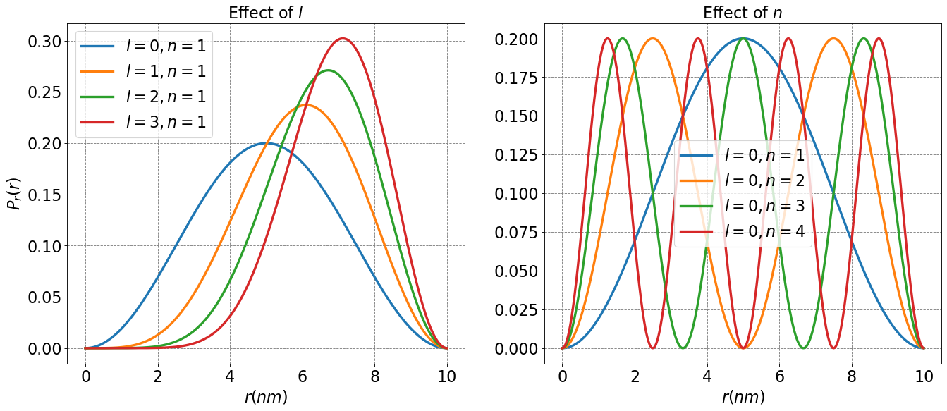
4.5.10.5. Particle Density

The probability density for quantum systems is defined as the complex conjugate of the wave function times the wave function. For a particle in a sphere this yields

(4.847)\[\begin{align} P(r,\theta,\phi) = \psi(r,\theta,\phi)^*\psi(r,\theta,\phi)r^2\sin\theta &= \frac{\left(2l+1\right)\left(l-|m|\right)!}{2\pi r_0^3\left(l+|m|\right)!} \frac{1}{j_{l+1}(\beta_{n,l})^2}j_l\left(\frac{\beta_{n,l}}{r_0}r\right)^2P_l^{|m|}(\cos\theta)^2r^2\sin\theta \end{align}\]

Notice that we include the \(r^2\sin\theta\) Jacobian in our definition of the probability density. It is because this must be included such that the integration over the probability density yields \(1\).

Additionally notice that the probability density is separable into \(r\), \(\theta\), and \(\phi\) components which allows us to define

(4.848)\[\begin{equation} P(r,\theta,\phi) = P_r(r)P_\theta(\theta)P_\phi(\phi) \end{equation}\]

where

(4.849)\[\begin{align} P_r(r) &= \frac{2}{r_0^3}\frac{1}{j_{l+1}(\beta_{n,l})^2} j_l\left(\frac{\beta_{n,l}}{r_0}r\right)r^2 \\ P_\theta(\theta) &= \frac{\left(2l+1\right)\left(l-|m|\right)!}{2 \left(l+|m|\right)!} P_l^{|m|}(\cos\theta)^2\sin\theta \\ P_\phi(\phi) &= \frac{1}{2\pi} \end{align}\]

We will now look at these individual components.

Show code cell source Hide code cell source

#### import numpy as np
import matplotlib.pyplot as plt
%matplotlib inline
from scipy.special import spherical_jn
def P_r(r,r0,n,l):
    zero_ln = spherical_jn_zero(l, n)
    return r_norm2(r0,n,l)*(spherical_jn(l, r*zero_ln/r0)*r)**2
def r_norm2(r0,n,l):
    zero_ln = spherical_jn_zero(l, n)
    return 2/(r0**3*spherical_jn(l+1, zero_ln)**2)
fontsize = 20
r = np.arange(0.0, 10.0, 0.01)
fig, ax = plt.subplots(1,2,figsize=(20,8),dpi= 80, facecolor='w', edgecolor='k')
ax[0].set_title(r'Effect of $l$', fontsize=fontsize)
ax[0].set_xlabel(r'$r (nm)$',size=fontsize)
ax[0].set_ylabel(r'$P_r(r)$',size=fontsize)
ax[0].tick_params(axis='both',labelsize=fontsize)
n = 1
for l in np.arange(4):
    ax[0].plot(r, P_r(r,10,n,l), lw = 3, label=rf'$l={l}, n={n}$')
ax[0].grid(b=True, which='major', axis='both', color='#808080', linestyle='--')
ax[0].legend(loc='best',fontsize=fontsize)
ax[1].set_title(r'Effect of $n$', fontsize=fontsize)
ax[1].set_xlabel(r'$r (nm)$',size=fontsize)
ax[1].tick_params(axis='both',labelsize=fontsize)
l = 0
for n in range(1,5):
    ax[1].plot(r, P_r(r,10,n,l), lw = 3, label=rf'$l={l}, n={n}$')
ax[1].grid(b=True, which='major', axis='both', color='#808080', linestyle='--')
ax[1].legend(loc='best',fontsize=fontsize)
plt.show();

/var/folders/td/dll8n_kj4vd0zxjm0xd9m7740000gq/T/ipykernel_32051/2044823888.py:21: MatplotlibDeprecationWarning: The 'b' parameter of grid() has been renamed 'visible' since Matplotlib 3.5; support for the old name will be dropped two minor releases later.
  ax[0].grid(b=True, which='major', axis='both', color='#808080', linestyle='--')
/var/folders/td/dll8n_kj4vd0zxjm0xd9m7740000gq/T/ipykernel_32051/2044823888.py:29: MatplotlibDeprecationWarning: The 'b' parameter of grid() has been renamed 'visible' since Matplotlib 3.5; support for the old name will be dropped two minor releases later.
  ax[1].grid(b=True, which='major', axis='both', color='#808080', linestyle='--')

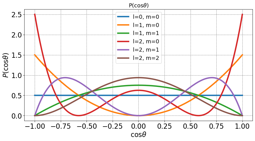
Show code cell source Hide code cell source

# plot of some of the Legendre polynomials
import warnings
warnings.filterwarnings('ignore')
import numpy as np
import matplotlib.pyplot as plt
%matplotlib inline
from scipy.special import lpmv

def P_theta(x,l,m):
    return theta_norm2(l,m)*lpmv(m,l,x)**2
def theta_norm2(l,m):
    return (2*l+1)*math.factorial(l-np.abs(m)) / (2*math.factorial(l+np.abs(m)))

x = np.arange(-1,1,0.0001)
plt.figure(figsize=(12,6),dpi= 80, facecolor='w', edgecolor='k')
plt.tick_params(axis='both',labelsize=20)
plt.grid(b=True, which='major', axis='both', color='#808080', linestyle='--')
for l in range(3):
    for m in range(0,l+1):
        label = "l=" + str(l) + ", m=" + str(m)
        plt.plot(x,P_theta(x,l,m),lw=4,label=label)
plt.title(r'P(cos$\theta$)',fontsize=16)
plt.xlabel(r'$\cos\theta$',size=fontsize)
plt.ylabel(r'$P(\cos\theta)$',size=fontsize)
plt.legend(fontsize=16);

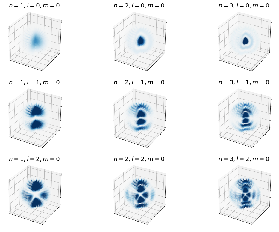
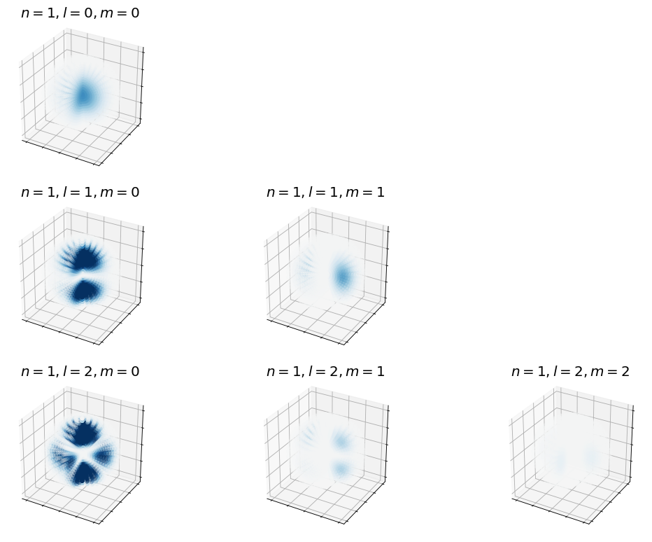
We can also look at them in 3D representations.

Show code cell source Hide code cell source

def particle_in_sphere_density(r,theta,phi,r0,n,l,m):
    return particle_in_sphere_wf(r,theta,phi,r0,n,l,m)**2

def plot_particle_in_sphere_density(n,l,m, ax_obj, r=np.linspace(0,1,15), theta=np.linspace(0,np.pi,20), phi=np.linspace(0,1.5*np.pi,25)):
    R, THETA, PHI = np.meshgrid(r, theta, phi)
    R = R.flatten()
    THETA = THETA.flatten()
    PHI = PHI.flatten()
    x = R*np.sin(THETA)*np.cos(PHI) 
    y = R*np.sin(THETA)*np.sin(PHI)
    z = R*np.cos(THETA)
    wf = particle_in_sphere_density(R,THETA,PHI,1.0,n,l,m)
    # plot
    ax_obj.set_title(rf'$n={n},l={l},m={m}$', fontsize=18)
    ax_obj.scatter3D(x,y,z,c=wf, cmap='RdBu', vmin=-0.2, vmax=0.2,alpha=0.25)
    ax_obj.set_box_aspect((100,100,100))
    #ax_obj.set_axis_off()
    ax_obj.axes.xaxis.set_ticklabels([])
    ax_obj.axes.yaxis.set_ticklabels([])
    ax_obj.axes.zaxis.set_ticklabels([])

Show code cell source Hide code cell source

fig, ax = plt.subplots(3,3,figsize=(16,12),dpi= 80, facecolor='w', edgecolor='k',subplot_kw={'projection': '3d'}) 
for l in range(3):
    for n in range(1,4):
        plot_particle_in_sphere_density(n,l,0,ax[l,n-1])
plt.show();

---------------------------------------------------------------------------
NameError                                 Traceback (most recent call last)
/var/folders/td/dll8n_kj4vd0zxjm0xd9m7740000gq/T/ipykernel_32051/3649633632.py in <module>
      2 for l in range(3):
      3     for n in range(1,4):
----> 4         plot_particle_in_sphere_density(n,l,0,ax[l,n-1])
      5 plt.show();

/var/folders/td/dll8n_kj4vd0zxjm0xd9m7740000gq/T/ipykernel_32051/12911347.py in plot_particle_in_sphere_density(n, l, m, ax_obj, r, theta, phi)
     10     y = R*np.sin(THETA)*np.sin(PHI)
     11     z = R*np.cos(THETA)
---> 12     wf = particle_in_sphere_density(R,THETA,PHI,1.0,n,l,m)
     13     # plot
     14     ax_obj.set_title(rf'$n={n},l={l},m={m}$', fontsize=18)

/var/folders/td/dll8n_kj4vd0zxjm0xd9m7740000gq/T/ipykernel_32051/12911347.py in particle_in_sphere_density(r, theta, phi, r0, n, l, m)
      1 def particle_in_sphere_density(r,theta,phi,r0,n,l,m):
----> 2     return particle_in_sphere_wf(r,theta,phi,r0,n,l,m)**2
      3 
      4 def plot_particle_in_sphere_density(n,l,m, ax_obj, r=np.linspace(0,1,15), theta=np.linspace(0,np.pi,20), phi=np.linspace(0,1.5*np.pi,25)):
      5     R, THETA, PHI = np.meshgrid(r, theta, phi)

/var/folders/td/dll8n_kj4vd0zxjm0xd9m7740000gq/T/ipykernel_32051/3767781050.py in particle_in_sphere_wf(r, theta, phi, r0, n, l, m)
      5 def particle_in_sphere_wf(r,theta,phi,r0,n,l,m):
      6     zero_ln = spherical_jn_zero(l, n)
----> 7     return A_nlm(n,l,m,r0)*sph_harm(m, l, phi, theta).real*spherical_jn(l, r*zero_ln/r0)

NameError: name 'sph_harm' is not defined

Show code cell source Hide code cell source

fig, ax = plt.subplots(3,3,figsize=(16,12),dpi= 80, facecolor='w', edgecolor='k',subplot_kw={'projection': '3d'}) 
for l in range(3):
    for m in range(3):
        if m <= l:
            plot_particle_in_sphere_density(1,l,m,ax[l,m])
        else: 
            ax[l,m].set_axis_off()
plt.show();

4.5.10.6. Average Properties

Now that we have normalized wave functions, it will be of interest to compute properties of these systems. These properties will be determined in the standard quantum mechanical way. For example, the average of some property \(a\) is given as

(4.850)\[\begin{align} \langle a \rangle &= \langle \psi(r,\theta,\phi) | \hat{A} | \psi(r,\theta,\phi)\rangle \\ &= \int_0^{r_0}\int_0^{\pi}\int_0^{2\pi} \psi_{nlm}^*(r,\theta,\phi)\hat{A}\psi_{nlm}(r,\theta,\phi)r^2\sin\theta drd\theta d\phi \end{align}\]

If the property does not couple two or more of the coordinates (i.e. if the property only depends on radial distance, angle in the xy plane, or azimuthal angle) then the integrals will still be separable and the problem should be less challenging than otherwise. Let’s look at the example of computing the average radial position for a particle in a sphere.

4.5.10.6.1. Average radial position

The average radial position is given by

(4.851)\[\begin{align} \langle r \rangle &= \langle \psi(r,\theta,\phi) | r | \psi(r,\theta,\phi)\rangle \\ &= \int_0^{r_0}\int_0^{\pi}\int_0^{2\pi} \psi_{nlm}^*(r,\theta,\phi)r\psi_{nlm}(r,\theta,\phi)r^2\sin\theta drd\theta d\phi \end{align}\]

Recognizing that we can integrate over \(\theta\) and \(\phi\) because the wave function is separable and the operator \(r\) does not affect \(\theta\) and \(\phi\), and that these functions are independently normalized quickly yields

(4.852)\[\begin{align} \langle r \rangle &= \frac{2}{r_0^3}\frac{1}{j_{l+1}(\beta_{n,l})^2}\int_0^{r_0} \left[j_l\left(\frac{\beta_{n,l}}{r_0}r\right)\right]^2r^3dr \\ &= \frac{2}{r_0^3}\frac{1}{j_{l+1}(\beta_{n,l})^2}r_0^4 \int_0^1 \left[j_l\left(\beta_{n,l}x\right)\right]^2x^3dx \\ &= \frac{2r_0}{j_{l+1}(\beta_{n,l})^2}\int_0^1 \left[j_l\left(\beta_{n,l}x\right)\right]^2x^3dx \end{align}\]

I am not sure if this can be simplified for general \(n\) and \(l\). An analytic solution for general \(n\) and \(l=0\) is left for an excercise. Here, I will use numeric intergration to look at the trends in increasing \(l\) and \(n\) on the average radial position.

Show code cell source Hide code cell source

# table of <r> for varying l and n
import numpy as np
from scipy.special import spherical_jn
from scipy.optimize import root
    
def r_integrand(r,n,l):
    zero_ln = spherical_jn_zero(l, n)
    r_norm = 2/spherical_jn(l+1, zero_ln)**2
    return r_norm*spherical_jn(l, zero_ln*r)**2*r**3
    
    
def spherical_jn_zero(l, n, ngrid=100):
    """Returns nth zero of spherical bessel function of order l
    """
    if l > 0:
        # calculate on a sensible grid
        x = np.linspace(l, l + 2*n*(np.pi * (np.log(l)+1)), ngrid)
        y = spherical_jn(l, x)
    
        # Find m good initial guesses from where y switches sign
        diffs = np.sign(y)[1:] - np.sign(y)[:-1]
        ind0s = np.where(diffs)[0][:n]  # first m times sign of y changes
        x0s = x[ind0s]
    
        def fn(x):
            return spherical_jn(l, x)

        return [root(fn, x0).x[0] for x0 in x0s][-1]
    else:
        return n*np.pi
print ("{:<8} {:<15} {:<20}".format('l','n','<r>'))
print("--------------------------------------------------------------------")
for l in range(4):
    for n in range(1,5):
        print ("{:<8} {:<15} {:<20}".format(l,n,np.round(integrate.quad(r_integrand,0,1,args=(n,l))[0],3)))    

l        n               <r>                 
--------------------------------------------------------------------
0        1               0.5                 
0        2               0.5                 
0        3               0.5                 
0        4               0.5                 
1        1               0.592               
1        2               0.539               
1        3               0.523               
1        4               0.515               
2        1               0.648               
2        2               0.574               
2        3               0.546               
2        4               0.532               
3        1               0.686               
3        2               0.603               
3        3               0.567               
3        4               0.548