4.3.1. The First Law of Thermodynamics#
Thermodynamics is the study of how heat moves. It tells us nothing about the time it takes for a process to happen but the laws of Thermodynamics have proven to govern whether things happen. Things can be anything from macroscopic phenomenon to biochemical processes.
4.3.1.1. Learning goals for today:#
After these notes, you should be able to:
Be able to state the first law of Thermodynamics
Define the internal energy of a chemical system
Define how a state function differs from a non-state function
Give at least three examples of state functions
Define a Thermodynamic system
4.3.1.2. Coding Concepts#
The following coding concepts are used in this notebook:
Numeric integration
Plotting with matplotlib
4.3.1.3. Statement of the first law#
The internal energy of an isolated system, \(U_{sys}\), is a state function and subject to conservation (\(\Delta U_{sys} = 0\) if the initial and final states are the same).
where an isolated system is one that cannot exchange heat or matter with surroundings, a state function has values that do not depend on the path taken, and \(\Delta U_{sys} = U_{sys}^{final} - U_{sys}^{initial}\)
4.3.1.4. Internal energy#
The internal energy of a chemical system is a measure of the chemical (potential) and thermal (kinetic) energy in the system. It is denoted internal because it does not include the kinetic and potential energies of the system moving as a whole or the interaction with the system and the surroundings. Within the context of chemistry, things like bond energies and the non-bonded interactions that we have discussed would be included in the internal energy.
4.3.1.5. State function#
State functions are important in Thermodynamics. These functions do not depend on path but only the initial and final position. Examples in Thermodynamics include change in internal energy (\(\Delta U\)), change in enthalpy (\(\Delta H\)), change in entropy (\(\Delta S\)), change in free energy (\(\Delta G\) or \(\Delta A\)), and others. State functions have the mathematical property of having an exact differential which will be important later on.
Examples of things that are not state functions: work, heat, and other specific forms of energy.
4.3.1.5.1. Example of a state function#
Consider going from point \(A\) to point \(B\) anywhere on the globe.
Elevation, \(Z\), is a state function: the elevations at points \(A\) and \(B\) only depend on where those points not how you got from point \(A\) to point \(B\). The change in elevation, \(\Delta Z\), is also then a state function.
Distance traveled is not a state function. There may be many different ways to get from point \(A\) to point \(B\) some of which will require traveling a greater distance. We say that distance traveled is path dependent.
4.3.1.5.2. Example of a State Function#
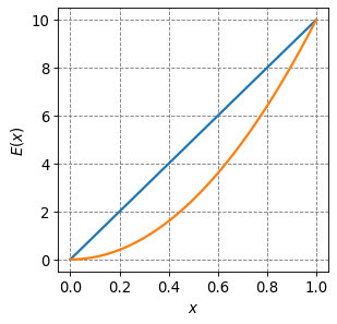
Consider going from and elevation of \(E(0) = 0\) to \(E(1)=10\) using two different paths:
\(E(x) = 10x\)
\(E(x) = 10x^2\)
Compute the change in elevation and distance traveled along these two paths.
# We start by plotting the two different paths
import numpy as np
import matplotlib.pyplot as plt
%matplotlib inline
# setup plot parameters
fontsize=12
fig = plt.figure(figsize=(4,4), dpi= 80, facecolor='w', edgecolor='k')
ax = plt.subplot(111)
ax.grid(b=True, which='major', axis='both', color='#808080', linestyle='--')
ax.set_xlabel("$x$",size=fontsize)
ax.set_ylabel("$E(x)$",size=fontsize)
plt.tick_params(axis='both',labelsize=fontsize)
# plot two curves
x = np.arange(0,1,0.0001)
plt.plot(x,10*x,lw=2)
plt.plot(x,10*x**2,lw=2)
[<matplotlib.lines.Line2D at 0x7f79226ef100>]
The change in elevation is clearly 10 in both cases but we will show that here.
For the first path:
For the second path:
For distance traveled, we need to compute path/arc length. This is easy enough for \(E_1\):
For the first path:
where we could also determine this using Pythagorean’s theorem.
For \(E_2\):
where I used numeric integration to estimate the last integral (see code below).
from scipy.integrate import quad
def integrand(x):
    return np.sqrt(1+400*x**2)
numeric_integral = quad(integrand,0,1)[0]
print(numeric_integral)
10.10472979397512
4.3.1.6. Thermodynamic system#
The concept of a system in Thermodynamics is somewhat vague but important. A system can be defined as anything but is typically the substance/volume of interest. This might be, for example, the beaker with the solution of interest during an experiment. Key concepts regarding a system are: definition of the system, surroundings and types of barriers between system and surroundings.
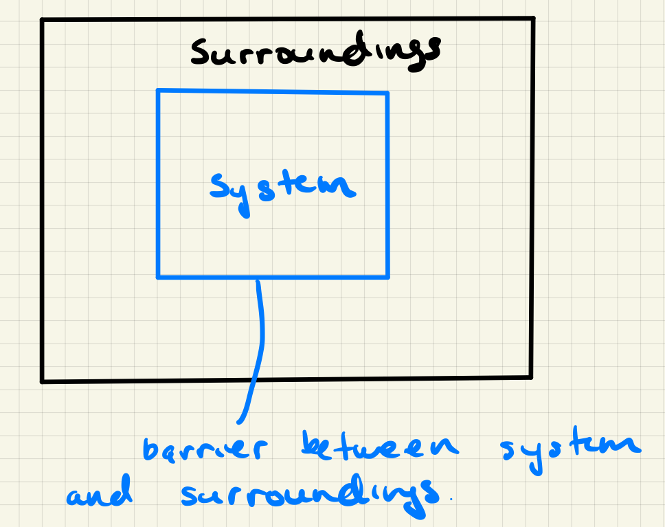
4.3.1.6.1. Types of Thermodynamic systems#
Isolated: An isolated system cannot transfer heat or mass between system and surroundings.
Closed: A closed system is one that cannot transfer mass between the system and the surroundings.
Open: An open system can transfer both heat and mass between the system and the surroundings.