3.1. Logarithms and Exponential Functions#
3.1.1. Learning goals:#
After working through these notes, you will be able to:
Evaluate exponential functions
Plot exponential functions
Manipulate exponential functions
Evaluate logarithmic functions
Plot logarithmic functions
Manipulate logarithmic functions
3.1.2. Coding concepts:#
The following coding concepts are used in this notebook:
3.1.3. Exponential Functions#
Exponential functions show up regularly in various areas of physical chemistry. Being comfortable manipulating and evaluating these types of functions is important. We start by evaluating and plotting exponential functions followed by revisiting the rules of algebraically manipulating these functions.
First, a definition, the exponential function is
This function takes the independent variable, \(x\), and raises \(e\) to this value to determine the dependent value, \(f(x)\).
3.1.3.1. Evaluating Exponential Functions#
Exponential functions are readily evaluated on any calculator or computer. For example, we might define
and ask, what is \(f(1.5)\)?
This will be evaluated by a computer/calculator. Below I do it using python code.
# import numpy library
import numpy as np
# define the function
def f(x):
    return 2*np.exp(3*x)
# print the specific value
print(f(1.5))
180.03426260104362
We can create more complicated exponential functions and evaluate their values at various \(x\) values. Here are some examples followed by the code to evaluate them.
import numpy as np
def f(x):
    return 1.2*np.exp(2*x+1)
def g(x):
    return 45*np.exp(-1.5*x)
def h(x):
    return 12.1*np.exp(-23*x+2)
print("f(3.2)=", f(3.2))
print("g(-2.0)=", g(-2.0))
print("h(0.01)=",h(0.01))
f(3.2)= 1963.1813159951123
g(-2.0)= 903.849161543445
h(0.01)= 71.03732567272948
3.1.3.2. Plotting Exponential Functions#
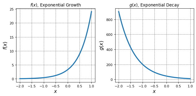
Exponential functions can be evaluated over the full domain of \(x\). If the largest power of \(x\) is positive then we will see exponential growth (the function will go to infinity as \(x\) goes to infinity) and if the largest power of \(x\) is negative then we will see exponential decay (the function will go to zero as \(x\) goes to infinity). We will plot one of each.
import matplotlib.pyplot as plt
%matplotlib inline
# setup plot
fontsize=14
fig,ax = plt.subplots(1,2,figsize=(8,4), dpi= 80, facecolor='w', edgecolor='k')
ax[0].grid(which='major', axis='both', color='#808080', linestyle='--')
ax[0].set_xlabel("$x$",size=fontsize)
ax[0].set_ylabel("$f(x)$",size=fontsize)
ax[0].set_title("$f(x)$, Exponential Growth")
x = np.arange(-2,1,0.001)
ax[0].plot(x,f(x),lw=3);
ax[1].grid(which='major', axis='both', color='#808080', linestyle='--')
ax[1].set_xlabel("$x$",size=fontsize)
ax[1].set_ylabel("$g(x)$",size=fontsize)
ax[1].set_title("$g(x)$, Exponential Decay")
x = np.arange(-2,1,0.001)
ax[1].plot(x,g(x),lw=3)
plt.tight_layout()
3.1.3.3. Manipulating Exponential Functions#
Exponential functions can be manipulated in various ways. Here are two common manipulations
Here is an example problem that uses both
Example: Show that
We start by using the reverse of the first rule above to combine everything into a single exponential
Now recognize that the quadratic function in the exponent is a perfect square so can be further simplified
We also have that natural log and exponential functions are inverse functions which means that
3.1.4. Logarithmic Functions#
Log functions are the inverse of exponential and/or power functions. These also come up frequently in physical chemistry and thus we must be able to evaluate, plot, and manipulate them.
An example logarthmic function is
where \(\ln\) stands for natural log or log base \(e\). We most commonly encounter natural logarithms so will not discuss other bases or change of bases in these notes but it is important to remember that these things exist.
It is also very important to consider the domain of logarithmic functions. The function \(f(x)=\ln(x)\) is only defined when \(x\) is greater than 0. That is, the function \(f(x)=\ln(x)\) is defined for \(x>0\).
3.1.4.1. Evaluating Logarithmic Functions#
Generally, we will use computers/calculators to evaluate logarithmic functions. For the function
there are some important things to remember, however:
Otherwise, evaluating logarthmic function is just a matter of entering it into your calculator. Here are some examples and the code to evaluate them.
import numpy as np
# Note: np.log is the natural log
def f(x):
    return 1.2*np.log(2*x+1)
def g(x):
    return 45*np.log(-1.5*x)
def h(x):
    return 12.1*np.log(-23*x+2)
print("f(3.2)=", f(3.2))
print("g(-2.0)=", g(-2.0))
print("h(0.01)=",h(-0.01))
f(3.2)= 2.401776000252149
g(-2.0)= 49.43755299006494
h(0.01)= 9.704219184211532
3.1.4.2. Plotting Logarithmic Functions#
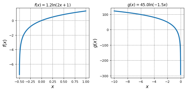
It is important to be able to plot these functions over their finite domains. Recall that the domain of a log function is determined by making the argument of the log greater than zero. You cannot take the log of zero or a negative number.
import matplotlib.pyplot as plt
%matplotlib inline
# setup plot
fontsize=14
fig,ax = plt.subplots(1,2,figsize=(8,4), dpi= 80, facecolor='w', edgecolor='k')
ax[0].grid(which='major', axis='both', color='#808080', linestyle='--')
ax[0].set_xlabel("$x$",size=fontsize)
ax[0].set_ylabel("$f(x)$",size=fontsize)
ax[0].set_title("$f(x)=1.2\ln(2x+1)$")
x = np.arange(-0.499,1,0.001)
ax[0].plot(x,f(x),lw=3);
ax[1].grid(which='major', axis='both', color='#808080', linestyle='--')
ax[1].set_xlabel("$x$",size=fontsize)
ax[1].set_ylabel("$g(x)$",size=fontsize)
ax[1].set_title("$g(x)=45.0\ln(-1.5x)$")
x = np.arange(-10,0,0.001)
ax[1].plot(x,g(x),lw=3)
plt.tight_layout();
3.1.4.3. Manipulating Logarithmic Functions (Rules of Logarithms)#
There are some important rules of logarithms that we should keep in mind:
And finally the fact that exponential and logarithmic functions are inverses yields