4.3.13. Maxwell Relations Applied

4.3.13.1. Learning goals:

After this section, student’s should be able to:

1. Identify the Maxwell relations

2. Utilize a Maxwell relation to calculate the change in internal energy of a non-ideal gas

3. Utilize a Maxwell relation to show enthalpy is independent of pressure for an ideal gas

4. Utilize a Maxwell relation to derive an expression for \(\Delta S\) of a van der Waals gas

5. Perform Legendre transforms and use Maxwell relations for a system with non-PV work

4.3.13.2. Coding concepts:

The following coding concepts are used in this notebook

1. Variables

2. Plotting with matplotlib

4.3.13.3. Maxwell Relations

4.3.13.3.1. Summary of Maxwell Relations

Energy Function	Differential Form $\( \)$	Maxwell Relations $\( \)$
U - Internal Energy	\( dU = TdS - PdV \)	\(\left(\frac{\partial T}{\partial V}\right)_S = -\left(\frac{\partial P}{\partial S}\right)_V\)
H - Enthalpy	\(dH = TdS + VdP\)	\(\left(\frac{\partial T}{\partial P}\right)_S = \left(\frac{\partial V}{\partial S}\right)_P\)
A - Helmholtz Free Energy	\(dA = -SdT - PdV\)	\(\left(\frac{\partial S}{\partial V}\right)_T = \left(\frac{\partial P}{\partial T}\right)_V\)
G - Gibbs Free Energy	\(dG = -SdT + VdP\)	\(\left(\frac{\partial S}{\partial P}\right)_T = -\left(\frac{\partial V}{\partial T}\right)_P\)

4.3.13.4. Example 1: Change in Internal Energy of a Non-Ideal Gas

Compute the change in internal energy, \(\Delta U\), for the isothermal expansion from \(V_1\) to \(V_2\) of a finite volume gas that has the equation of state:

\(P(V-nb) = nRT\)

Recall that for an ideal gas we always used the relationship \(\Delta U_{ideal} = n\bar{C}_V\Delta T\) and thus the change in internal energy for an ideal gas is zero for an isothermal process. But what about this non-ideal gas?

In order to compute \(\Delta U\), we start with the differential form of the internal energy

(4.329)\[\begin{align} dU = TdS - PdV \end{align}\]

Integrate both sides to yield

(4.330)\[\begin{align} \Delta U = \int_{U_i}^{U_f}dU = \int_{S_i}^{S_f} TdS - \int_{V_i}^{V_f}PdV \end{align}\]

Notice that we can handle the second term, \(\int_{V_i}^{V_f}PdV\), by plugging in the equation of state for our finite volume gas but the first term, \(\int_{S_i}^{S_f} TdS\), is a bit harder to handle; while \(T\) is constant we do not know the change in entropy.

Solution: change the integration variable using a Maxwell relation. Given that we know initial and final volumes, and that the second integral is with resepct to volume, we would really like to change the \(dS\) to a \(dV\). For this, we look at the Maxwell Relations and pick the one that has \(\left(\frac{\partial S}{\partial V}\right)\) and ideally at contsant \(T\) since our process is isothermal:

Energy Function	Differential Form $\( \)$	Maxwell Relations $\( \)$
U - Internal Energy	\( dU = TdS - PdV \)	\(\left(\frac{\partial T}{\partial V}\right)_S = -\left(\frac{\partial P}{\partial S}\right)_V\)
H - Enthalpy	\(dH = TdS + VdP\)	\(\left(\frac{\partial T}{\partial P}\right)_S = \left(\frac{\partial V}{\partial S}\right)_P\)
A - Helmholtz Free Energy	\(dA = -SdT - PdV\)	\(\left(\frac{\partial S}{\partial V}\right)_T = \left(\frac{\partial P}{\partial T}\right)_V\)
G - Gibbs Free Energy	\(dG = -SdT + VdP\)	\(\left(\frac{\partial S}{\partial P}\right)_T = -\left(\frac{\partial V}{\partial T}\right)_P\)

We see that the Maxwell Relation from \(A\) is

\(\left(\frac{\partial S}{\partial V}\right)_T = \left(\frac{\partial P}{\partial T}\right)_V\)

The goal is now to rerrange this partial derivative to get \(dS\) as a function of \(dV\). To do this, we “cross multiply” by \(dV\):

(4.331)\[\begin{align} \left(\frac{\partial S}{\partial V}\right)_T =& \left(\frac{\partial P}{\partial T}\right)_V \\ \Rightarrow dS = & \left(\frac{\partial P}{\partial T}\right)_V dV \end{align}\]

Note that even though the derivative infront of \(dV\) is taken at constant \(V\), the resulting function could still be dependent on \(V\).

Now, let’s plug this into our \(\Delta U\) equation:

(4.332)\[\begin{align} \Delta U =& \int_{S_i}^{S_f} TdS - \int_{V_i}^{V_f}PdV \\ =& \int_{V_i}^{V_f} T\left(\frac{\partial P}{\partial T}\right)_V dV - \int_{V_i}^{V_f}PdV \\ =& \int_{V_i}^{V_f} \left[ T\left(\frac{\partial P}{\partial T}\right)_V -P\right]dV \\ \end{align}\]

Now we need to determine \(\left(\frac{\partial P}{\partial T}\right)_V\), plug back into the integrand, and perform the integration.

(4.333)\[\begin{align} \left(\frac{\partial P}{\partial T}\right)_V =& \frac{\partial}{\partial T} \left( \frac{nRT}{V-nb}\right) \\ =& \frac{nR}{V-nb} \end{align}\]

Now plug back into integral:

(4.334)\[\begin{align} \Delta U =& \int_{V_i}^{V_f} \left[ T\left(\frac{\partial P}{\partial T}\right)_V -P\right]dV \\ =& \int_{V_i}^{V_f} \left[ T\frac{nR}{V-nb} -\frac{nRT}{V-nb}\right]dV \\ =& 0 \end{align}\]

So we did all of that to see that the change in internal energy of a finite volume gas for an isothermal process is zero, just like it is for an ideal gas (which you could also show using a very similar derivation).

4.3.13.5. Example 2: Enthalpy and Pressure for an ideal gas

Show that the enthlapy of an ideal gas is independent of pressure under isothermal conditions.

We start with the differential form of enthalpy

(4.335)\[\begin{align} dH =& TdS + VdP \\ \Rightarrow \Delta H =& \int_{H_i}^{H_f}dH = \int_{S_i}^{S_f}TdS + \int_{P_i}^{P_f}VdP \\ \end{align}\]

Again, the second integral on the right-hand side of the equation is managable because we know the equation of state for an ideal gas. The first integral requires us to know entropy change which is not readily known. Thus, we would like to convert the integral with respect to \(S\) to and integral with respect to \(P\) (to match with the second integral).

Again, we consult our Maxwell relations look for a \(\frac{\partial S}{\partial P}\) term

Energy Function	Differential Form $\( \)$	Maxwell Relations $\( \)$
U - Internal Energy	\( dU = TdS - PdV \)	\(\left(\frac{\partial T}{\partial V}\right)_S = -\left(\frac{\partial P}{\partial S}\right)_V\)
H - Enthalpy	\(dH = TdS + VdP\)	\(\left(\frac{\partial T}{\partial P}\right)_S = \left(\frac{\partial V}{\partial S}\right)_P\)
A - Helmholtz Free Energy	\(dA = -SdT - PdV\)	\(\left(\frac{\partial S}{\partial V}\right)_T = \left(\frac{\partial P}{\partial T}\right)_V\)
G - Gibbs Free Energy	\(dG = -SdT + VdP\)	\(\left(\frac{\partial S}{\partial P}\right)_T = -\left(\frac{\partial V}{\partial T}\right)_P\)

We choose the following Maxwell relation

(4.336)\[\begin{align} \left(\frac{\partial S}{\partial P}\right)_T &= -\left(\frac{\partial V}{\partial T}\right)_P \end{align}\]

from the Gibbs free energy row. Rearrange that equation to get

(4.337)\[\begin{align} dS &= -\left(\frac{\partial V}{\partial T}\right)_PdP \end{align}\]

Plug back into the integral

(4.338)\[\begin{align} \Delta H &= \int_{S_i}^{S_f}TdS + \int_{P_i}^{P_f}VdP \\ &= \int_{P_i}^{P_f} \left[ -T\left(\frac{\partial V}{\partial T}\right)_P + V\right]dP \end{align}\]

Using the equation of state (\(PV=nRT\)), we will solve for \(\left(\frac{\partial V}{\partial T}\right)_P\):

(4.339)\[\begin{align} \left(\frac{\partial V}{\partial T}\right)_P &= \frac{\partial}{\partial T}\left(\frac{nRT}{P}\right) \\ &= \frac{nR}{P} \end{align}\]

Plug back into the integral and substitute \(V = \frac{nRT}{P}\) to see:

(4.340)\[\begin{align} \Delta H &= \int_{P_i}^{P_f} \left[ -T\left(\frac{\partial V}{\partial T}\right)_P + V\right]dP \\ &=\int_{P_i}^{P_f} \left[ -T\frac{nR}{P} + \frac{nRT}{P}\right]dP \\ &= 0 \end{align}\]

4.3.13.6. Example 3: Compute \(\Delta S\) a reversible isothermal expansion of a non-ideal gas

Consider a van der Waals gas with the equation of state

(4.341)\[\begin{equation} P = \frac{nRT}{V-nb} - \frac{an^2}{V^2} \end{equation}\]

Compute the change in entropy, \(\Delta S\), during a reversible isothermal expansion of this gas.

For this we start with the Maxwell relation

(4.342)\[\begin{equation} \left(\frac{\partial S}{\partial V}\right)_T = \left(\frac{\partial P}{\partial T}\right)_V \end{equation}\]

Which can be rearranged to yield

(4.343)\[\begin{equation} dS = \left(\frac{\partial P}{\partial T}\right)_V dV \quad \text{constant T} \end{equation}\]

Integrating both sides will yield the desired solution. We start by computing the partial derivative of \(P\) w.r.t. \(T\) from the equation of state:

(4.344)\[\begin{equation} \left(\frac{\partial P}{\partial T}\right)_V = \frac{nR}{V-nb} \end{equation}\]

Now plug-in and do the integral w.r.t. V:

(4.345)\[\begin{eqnarray} \Delta S &=& \int_{V_1}^{V_2} \frac{nR}{V-nb} dV \\ &=& nR \ln\left( \frac{V_2-nb}{V_1-nb}\right) \end{eqnarray}\]

4.3.13.7. Example 4: System with non-PV work

Consider a system composed of a stretchable/elastic solid. The energy associated with stretching the solid is given as

(4.346)\[\begin{equation} FdL \end{equation}\]

where \(F\) is the elastic coefficient of the system and \(L\) is the length of the material. In this case, the differential of internal energy, for example, is given as

(4.347)\[\begin{equation} dU = TdS - PdV + FdL \end{equation}\]

(a) Derive an expression for \(dD\) where \(D = A-FL\) is a new thermodynamic energy function.

(b) Describe how you might measure the change in entropy w.r.t force for this system at constant \(V\) and \(T\).

Part (a) is essentially asking us to perform a Legendre transform of \(A\) to achieve a new function \(D\) that swaps natural variales \(F\) and \(L\).

(4.348)\[\begin{eqnarray} D &=& A - FL \\ \Rightarrow dD &=& dA - FdL - LdF \\ &=& -SdT - PdV + FdL - FdL - LdF \\ &=& -SdT - PdV - LdF \end{eqnarray}\]

From this expression we have the following Maxwell relation (among others)

(4.349)\[\begin{equation} \left( \frac{\partial S}{\partial F}\right)_{T,V} = \left( \frac{\partial L}{\partial T}\right)_{V,F} \end{equation}\]

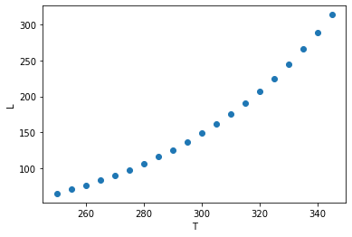
This equation states that the change in entropy with respect to force (\(F\)) is equal to the change in length of the material with respect to temperature (at constant force). So you could measure the length of the material under constant volume and force conditions for various temperatures to estimate how entropy varies with respect to force.

import matplotlib.pyplot as plt
%matplotlib inline
import numpy as np

T = np.arange(250,350,5.0)
L = np.exp(T/60)
plt.plot(T,L,'o')
plt.xlabel("T")
plt.ylabel("L")

Text(0, 0.5, 'L')