4.5.15. The Helium Atom#
4.5.15.1. Motivation#
We have determined the energies and wave functions of the hydrogen atom and hydrogen-like ions. In these notes, we will determine the energies and wave functions for the helium atom (a multi-electron atom).
4.5.15.2. Learning Goals:#
After working through these notes, you will be able to:
Write out the Hamiltonian for the helium atom.
Use first order perturbation theory to solve for the approximate energy of the helium atom.
Use the variational method to solve for the approximate energy of the helium atom.
Use the variational method to solve for the approximate ground-state wave function of the helium atom.
4.5.15.3. Coding Concepts:#
The following coding concepts are used in this notebook:
4.5.15.4. The Model of the Helium Atom#
The helium atom is composed of a two electrons, two protons and two neutrons. If these particles were classical, the interaction energy would be the Coulombic attraction between electron and the nuclei as well as the Coulombic repulsion between the two electrons (assuming the protons and neutrons reside at a single stationary point):
\(V(\vec{r_1},\vec{r_2}) = -\frac{2e^2}{4\pi\epsilon_0|\vec{r_1}|}-\frac{2e^2}{4\pi\epsilon_0|\vec{r_2}|} + \frac{e^2}{4\pi\epsilon_0|\vec{r_1}-\vec{r_2}|}\),
where \(\vec{r_1}\) is the separation vector between the electron 1 and the nucleus, \(r_2\) is the separation vector between electron 2 and the nucleus, \(e\) is the charge of an electron and \(\epsilon_0\) is the permittivity of free space. In atomic units the potential simply becomes
\(V(\vec{r_1},\vec{r_2}) = -\frac{2}{|\vec{r_1}|}-\frac{2}{|\vec{r_2}|} + \frac{1}{|\vec{r_1}-\vec{r_2}|}\).
In the quantum mechanical picture, we will treat this same function as the potential energy operator. The Hamiltonian in atomic units for a helium atom is then, including the kinetic energy,
\(\hat{H}(\vec{r_1},\vec{r_2}) = -\frac{1}{2}\nabla_1^2-\frac{1}{2}\nabla_2^2-\frac{2}{|\vec{r_1}|}-\frac{2}{|\vec{r_2}|} + \frac{1}{|\vec{r_1}-\vec{r_2}|}\)
where \(\nabla_i^2\) is the Laplacian for particle \(i\) in three dimensions. We can rearrange the right hand side of the above equation to yield
\(\hat{H}(\vec{r_1},\vec{r_2}) = -\frac{1}{2}\nabla_1^2-\frac{2}{|\vec{r_1}|}-\frac{1}{2}\nabla_2^2-\frac{2}{|\vec{r_2}|} + \frac{1}{|\vec{r_1}-\vec{r_2}|}\)
\( = \hat{H}^{Z=2}_H(\vec{r_1}) + \hat{H}^{Z=2}_H(\vec{r_2}) + \frac{1}{r_{12}}\),
where \(\hat{H}^{Z=2}_H(\vec{r_i})\) is the Hydrogen-like Hamiltonian for particle \(i\) with a nuclear charge of 2\(e\) and \(r_{12} = |\vec{r_1}-\vec{r_2}|\) .
The Schrodinger equation for the Helium atom cannot be solved analytically. We will show how to approximate the ground-state energy using first-order perturbation theory and the variational approach.
4.5.15.5. First-order Perturbation Theory#
To apply first-order perturbation theory we must divide the Hamiltonian into a zeroth-order Hamiltonian plus a perturbation. Here we treat the electron-electron repulsion as the perturbation (not a great approximation as we will see)
\(\hat{H}(\vec{r_1},\vec{r_2}) = \hat{H}^0 + \hat{H}^1\),
where
\(\hat{H}^0 = \hat{H}^{Z=2}_H(\vec{r_1}) + \hat{H}^{Z=2}_H(\vec{r_2})\)
and
\(\hat{H}^1 = \frac{1}{r_{12}}\).
In first-order perturbation theory, the total energy of the system is approximated as the eigenvalue of the zeroth-order Schrodinger equation plus the expectation value of the perturbation in the zeroth-order wavefunctions. The zeroth-order wavefunction is the solution to the Schrodingder equation
\(H^0(\vec{r_1},\vec{r_2}) \psi^0(\vec{r_1},\vec{r_2})= E^0\psi^0(\vec{r_1},\vec{r_2})\).
Since we can write the Hamiltonian here as a sum of independent hydrogen-like Hamiltonians, the wavefunctions (eigenfunctions of this Hamiltonian) are products of hydrogen-like wavefunctions
\(\psi^0(\vec{r_1},\vec{r_2}) = \phi_{1s}^{Z=2}(\vec{r_1})\phi_{1s}^{Z=2}(\vec{r_2})\),
where
\(\phi_{1s}^{Z}(\vec{r_1}) = \frac{Z^{3/2}}{\sqrt{\pi}}e^{-Z|\vec{r_1}|}\)
can be determined by analogy to the hydrogen atom wave functions. The zeroth order energy is then a sum of hydrogen-like energies
\(E^0 = -\frac{Z^2}{2} - \frac{Z^2}{2} = -Z^2 = -4\) Hartree.
First order perturbation theory dictates that
This integral is quite a pain to evaluate but works out to be
Finally, we get the total energy of the helium atom by adding \(E^0\) and \(E^1\):
4.5.15.6. Variational Approach#
The variational principle applied to the Schrodinger equation yields that if
\(\hat{H}\psi_0 = E_0\psi_0\)
is the Schrodinger equation for the Hamiltonian of interest then
\(E_\phi = \frac{\langle\phi|\hat{H}|\phi\rangle}{\langle\phi|\phi\rangle} > E_0\)
for any function \(\phi\neq\psi_0\).
How does this help us in practice? In a typical QM problem, we are attempting to solve for the wavefunction(s) and energy(ies) for a given Hamiltonian. If the Hamiltonian is such that solving the problem exactly is too challenging (e.g. any two or more electron problem) we can expand the wavefunction in a basis and attempt to solve the problem that way. We start with
\(\psi \approx \phi = \sum_n^N c_nf_n\).
Truncating this expansion at any finite \(n\) leads to an approximate solution. Also, what the variational principle tells us is that we can minimize the energy with respect to variational paramters \({c_n}\) and still have \(E_\phi \geq E_0\).
For the helium atom, we will propose a trial wave function that is simply a product of the two hydrogen-like 1s orbitals, just like the zeroth order wave functions we used in the perturbation theory approximation above. The difference is that we will use the effective nuclear charge as the variational parameter. That is, we posit a trial wave function
\(\psi_t(r_1,r_2) = \frac{\zeta^3}{\pi}e^{-\zeta(r_1+r_2)}\),
due to this being a product of two Hydrogen 1s like orbitals and \(\zeta\) is our variational parameter. The first step in the variational approach is to solve for the expectation value of the Hamiltonian in this trial wavefunction. It can be shown that
\(\langle E \rangle_t = \frac{ \langle \psi_t | \hat{H} | \psi_t \rangle}{\langle \psi_t | \psi_t \rangle} = \zeta^2 - \frac{27}{8}\zeta\)
We then minimize \(\langle E \rangle_t\) with respect to the variational parameter
\(\frac{d \langle E \rangle_t}{d\zeta}|_{\zeta_{min}} = 0\)
\(\Rightarrow \zeta_{min} = \frac{27}{16}\)
\(\Rightarrow E_{min} = -2.8477\) Hartree
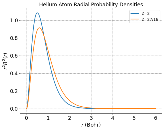
The variationally optimal approximation to the wave function is thus \(\psi_t(r_1,r_2) = \frac{\left(\frac{27}{16}\right)^3}{\pi}e^{-\frac{27}{16}(r_1+r_2)}\). A single 1s orbital with this effective nuclear charge is plotted below as a function of separation distance between the electron and nucleus. It is compared to the 1s with a charge of 2e.
Show code cell source
# let's plot some radial wavefunctions of the hydrogen atom
from scipy.special import sph_harm
from scipy.special import eval_genlaguerre
from scipy.special import factorial
from scipy import integrate
import numpy as np
import matplotlib.pyplot as plt
%matplotlib inline

fontsize = 16
plt.figure(figsize=(8,6),dpi= 80, facecolor='w', edgecolor='k')
plt.tick_params(axis='both',labelsize=fontsize)
plt.grid(which='major', axis='both', color='#808080', linestyle='--')
plt.title("Helium Atom Radial Probability Densities",fontsize=fontsize)
plt.ylabel(r'$r^2R^2(r)$',size=fontsize)
plt.xlabel(r'$r$ (Bohr)',size=fontsize)

# parameters for plotting
nLimit = 1
a0 = 1.0
r = np.arange(0,6,0.01)
Z = 2
n=1
l=0
prefactor = -np.sqrt(factorial(n-l-1)/(2*n*factorial(n+l)))*(2.0*Z/(n*a0))**(l+1.5)*np.power(r,l)*np.exp(-Z*r/(n*a0))
R = prefactor*eval_genlaguerre(n-l-1,2*l+1,2*Z*r/(n*a0))
label = "Z=2"
plt.plot(r,np.power(R,2)*np.power(r,2),label=label, lw=2)
Z = 27/16
prefactor = -np.sqrt(factorial(n-l-1)/(2*n*factorial(n+l)))*(2.0*Z/(n*a0))**(l+1.5)*np.power(r,l)*np.exp(-Z*r/(n*a0))
R = prefactor*eval_genlaguerre(n-l-1,2*l+1,2*Z*r/(n*a0))
label = "Z=27/16"
plt.plot(r,np.power(R,2)*np.power(r,2),label=label, lw=2)
plt.legend(fontsize=12)
plt.show();
4.5.15.7. Comparison of the Two Methods#
Perturbation theory yields a ground-state energy for the helium atom as
The variational method (with the specific basis functions that we chose) yields
These can be compared to the experimental value of
From this comparison we see that the variational solution yields a value closer to experiment that perturbation theory. This shouldn’t be all that surprising since the assumption that the perturbation is small is not a good one.
As a final, practical, point of comparison, the variational approach yields approximate wave functions and this is something that is not (easily) achievable with perturbation theory.