Thermodynamic Cycles: Solving exam problems and other examples

4.3.5. Thermodynamic Cycles: Solving exam problems and other examples#

4.3.5.1. Learning Goals#

After this lesson, you should be able to:

Set up thermodynamic problems and solve them quickly in an exam setting.
Solve for pressure, volume, and temperature relationships on a thermodynamic cycle.
Solve for work, heat, change in internal energy, and change in enthalpy for a thermodynamic cycle process.
Compare extractable work from a process with an adiabat or isotherm.

4.3.5.2. Tips for solving thermodynamic cycle exam problems#

Follow these tips to solve thermodynamic cycle problems faster during an exam when time is limited.

Use or a make a table that lists each process and the initial and final values for pressure, temperature, and volume. Clearly identify initial and final values rather than using \(V_1\) or \(V_2\) to make plugging values into equations easier.
Set up a blank table with each process listed and all the thermodynamic values you need to solve for.
Add any values you are given into the table.
Fill in any ‘zero’ values. For example, no work is extracted from an isochoric process and no heat from an adiabat.
Set up a total row. State functions, such as \(\Delta\) \(U\) and \(\Delta\) \(H\), sum to zero in a cycle.
Use the relationship \(w + q = \Delta U\). For an isotherm, \(\Delta\) \(U\) is zero so you can quickly find \(w\) and \(q\) by only solving for one and the other one must be equal in magnitude and opposite.

Take advantage of the relationships in steps 4 and 5 to avoid plugging in and solving for each value. These relationships can also be used to check your work.

4.3.5.3. Cycle A: Adiabatic, Isobaric, Isochoric#

This 3 membered cycle begins with an adiabatic compression, then isobaric compression, and isochoric heating. We are given \(n\) = 1, \(V_1\) = 2.0 L, \(V_2\) = 8.0 L, and \(T_1\) = 300.0 K. To solve for \(P_1\), \(P_2\), and \(T_2\) we will need to use adiabatic relationships and the ideal gas law.

../../_images/ee216098a7b4860d08cc92462d6445cd561df0eb1068d9ffc31453bbe8f7d7e4.png

4.3.5.3.1. Solving for P, V, T on Cycle A#

To solve for \(P_1\), use \(T_1\), \(V_1\), and the ideal gas law.

(4.213)#\[\begin{align} P_1 &= \frac{nRT_1}{V_1} \\ &= \frac{0.08206\cdot300}{2} \\ &= 12.3 \text{ atm} \end{align}\]

Use an adiabatic relationship to solve for \(T_2\). At any point along the curve, \(PV^{5/3}\) is constant.

(4.214)#\[\begin{align} P_1V_1^{5/3} &= P_2V_2^{5/3} \\ \Rightarrow P_2 &= P_1\cdot\left(\frac{V_1}{V_2}\right)^\frac{5}{3} \\ &= 12.3\cdot\left(\frac{2}{8}\right)^\frac{5}{3} \\ &= 1.2 \text{ atm} \end{align}\]

To solve for \(T_2\) use the ideal gas law and the values for \(V_2\) and \(P_2\).

(4.215)#\[\begin{align} T_2 &= \frac{P_2V_2}{nR} \\ &= \frac{1.2\cdot8}{0.08206} \\ &= 118.9 \text{ K} \end{align}\]

To solve for \(T_3\) use the ideal gas law and the values for \(V_1\) and \(P_2\).

(4.216)#\[\begin{align} T_3 &= \frac{P_2V_1}{nR} \\ &= \frac{1.2\cdot2}{0.08206} \\ &= 29.7 \text{ K} \end{align}\]

Below is a table of values for Cycle A.

Process	\(V_i\) (L)	\(V_f\) (L)	\(P_i\) (atm)	\(P_f\) (atm)	\(T_i\) (K)	\(T_f\) (K)
Adiabatic	2.0	8.00	12.3	1.2	300.0	118.9
Isobaric	8.0	2.0	1.2	1.2	118.9	29.7
Isochoric	2.0	2.0	1.2	12.3	29.7	300.0

4.3.5.3.2. Solving for work, heat, change in internal energy, and change in enthalpy on Cycle A#

We will calculate values for work, heat, change in internal energy, and change in enthalpy using the following equations.

Process	\(w\)	\(q\)	\(\Delta\) U	\(\Delta\) H
Adibatic	\(\frac{3}{2}nR(T_f-T_i)\)	\(0\)	\(\frac{3}{2}nR(T_f-T_i)\)	\(\frac{5}{2}nR(T_f-T_i)\)
Isobaric	\(-(\frac{nRT_f}{V_f})\Delta V\)	\(\Delta U - w\)	\(\frac{3}{2}nR(T_f-T_i)\)	\(\frac{5}{2}nR(T_f-T_i)\)
Isochoric	\(0\)	\(\frac{3}{2}nR(T_i-T_f)\)	\(\frac{3}{2}nR(T_f-T_i)\)	\(\frac{5}{2}nR(T_f-T_i)\)
Total	\(\frac{3}{2}nR(T_f-T_i)-(\frac{nRT_f}{V_f})\Delta V\)	\(-\frac{3}{2}nR(T_f-T_i)+(\frac{nRT_f}{V_f})\Delta V\)	\(0\)	\(0\)

4.3.5.3.2.1. Adiabat#

We want to solve for \(w\), \(q\), \(\Delta\) \(U\), and \(\Delta\) \(H\) from \((V_1, P_1, T_1)\) to \((V_2, P_2, T_2)\).

(4.217)#\[\begin{align} q &= 0 \\ \\ w &= \frac{3}{2}nR(T_f-T_i) \\ &= \frac{3}{2}\cdot0.08206(118.9-300) \\ &= -22.3 \text{ L atm}\\ \\ \Delta U &= w \\ &= -22.3 \text{ L atm}\\ \\ \Delta H &= \frac{5}{2}nR(T_f-T_i) \\ &= \frac{5}{2}\cdot0.08206(118.9-300) \\ &= -37.2 \text{ L atm}\\ \end{align}\]

4.3.5.3.2.2. Isobaric#

We want to solve for \(w\), \(q\), \(\Delta\) \(U\), and \(\Delta\) \(H\) from \((V_2, P_2, T_2)\) to \((V_1, P_2, T_3)\).

(4.218)#\[\begin{align} w &= -(\frac{nRT_f}{V_f})\Delta V \\ &= -(\frac{0.08206\cdot29.7}{2})(2-8) \\ &=7.3 \text{ L atm}\\ \\ \Delta U &= \frac{3}{2}nR(T_f-T_i) \\ &= \frac{3}{2}\cdot0.08206(29.7-118.9) \\ &= -11.0 \text{ L atm}\\ \\ q &= \Delta U - w \\ &= -18.3 \text{ L atm}\\ \\ \Delta H &= \frac{5}{2}nR(T_f-T_i) \\ &= \frac{5}{2}\cdot0.08206(29.7-118.9) \\ &= -18.3 \text{ L atm} \end{align}\]

4.3.5.3.2.3. Isochoric#

We want to solve for \(w\), \(q\), \(\Delta\) \(U\), and \(\Delta\) \(H\) from \((V_1, P_2, T_2)\) to \((V_1, P_1, T_1)\).

(4.219)#\[\begin{align} w &= 0 \\ \\ \Delta U &= \frac{3}{2}nR(T_f-T_i) \\ &= \frac{3}{2}\cdot0.08206(300-29.7) \\ &= 33.3 \text{ L atm}\\ \\ q &= \Delta U \\ &= 33.3 \text{ L atm}\\ \\ \Delta H &= \frac{5}{2}nR(T_f-T_i) \\ &= \frac{5}{2}nR(300-29.7) \\ &= 55.5 \text{ L atm} \end{align}\]

Process	\(w\) (L atm)	\(q\) (L atm)	\(\Delta\) \(U\) (L atm)	\(\Delta\) \(H\) (L atm)
A Adiabatic	-22.3	0	-22.3	-37.2
B Isobaric	7.3	-18.3	-11.0	-18.3
C Isochoric	0	33.3	33.3	55.5
Total	-15	15	0	0

4.3.5.4. Cycle B: Isotherm, Isochoric, and Isobaric#

This 3 membered cycle begins with an isothermal compression, then isobaric compression, and isochoric heating. We are given \(n\) = 1, \(V_1\) = 2.0 L, \(V_2\) = 8.0 L, and \(T_1\) = 300.0 K.

../../_images/3aaf7dbd5f4a3fdcc637e6a4aefd90afd9233b81e41bff36467b5f764a4e1c56.png

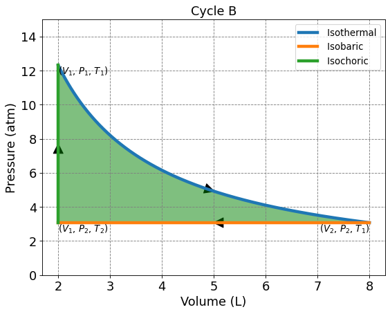
4.3.5.4.1. Solving for P, V, and T on Cycle B#

Use the ideal gas law and the provided values to solve for \(P_1\).

(4.220)#\[\begin{align} P_1 &= \frac{nRT_1}{V_1} \\ &= \frac{0.08206\cdot300}{2} \\ &= 12.3 \text{ atm} \\ \end{align}\]

Temperature is constant along an isotherm. Use the ideal gas law, \(V_2\), and \(T_1\) to solve for \(P_2\).

(4.221)#\[\begin{align} P_2 &= \frac{nRT_1}{V_2} \\ &= \frac{0.08206\cdot300}{8} \\ &= 3.1 \text{ atm} \end{align}\]

\(T_2\) can be solved using the ideal gas law, \(V_1\), and \(P_2\).

(4.222)#\[\begin{align} T_2 &= \frac{P_2V_1}{nR} \\ & = \frac{3.1\cdot2}{0.08206} \\ &= 75.6 \text{ K} \end{align}\]

Process	\(V_i\) (L)	\(V_f\) (L)	\(P_i\) (atm)	\(P_f\) (atm)	\(T_i\) (K)	\(T_f\) (K)
Isotherm	2.0	8.0	12.3	3.1	300.0	300.0
Isobaric	8.0	2.0	3.1	3.1	300.0	75.6
Isochoric	2.0	2.0	3.1	12.3	75.6	300.0

4.3.5.4.2. Solving for work, heat, change in internal energy, and change in enthalpy on Cycle B#

Process	\(w\)	\(q\)	\(\Delta\) \(U\)	\(\Delta\) \(H\)
Isothermal	\(nRT_f\ln\left(\frac{V_i}{V_f}\right)\)	\(nRT_f\ln\left(\frac{V_f}{V_i}\right)\)	\(0\)	\(0\)
Isobaric	\(-(\frac{nRT_f}{V_f})\Delta V\)	\(\Delta U - w\)	\(\frac{3}{2}nR(T_f-T_i)\)	\(\frac{5}{2}nR(T_f-T_i)\)
Isochoric	\(0\)	\(\frac{3}{2}nR(T_i-T_f)\)	\(\frac{3}{2}nR(T_f-T_i)\)	\(\frac{5}{2}nR(T_f-T_i)\)
Total	\(nRT_f\ln\left(\frac{V_i}{V_f}\right)-(\frac{nRT_f}{V_f})\Delta V\)	\(-nRT_f\ln\left(\frac{V_i}{V_f}\right)+(\frac{nRT_f}{V_f})\Delta V\)	\(0\)	\(0\)

4.3.5.4.2.1. Isotherm#

We want to solve for \(w\), \(q\), \(\Delta\) \(U\), and \(\Delta\) \(H\) from \((V_1, P_1, T_1)\) to \((V_2, P_2, T_1)\).

Along an isotherm, temperature is constant which is why \(\Delta\) \(U\) and \(\Delta\) \(H\) are 0.

(4.223)#\[\begin{align} \Delta U &= 0 \\ \Delta H &= 0 \\ \end{align}\]

To calulate work and heat use the equations that have been derived in previous notebooks.

(4.224)#\[\begin{align} w &= nRT_2\ln(\frac{V_i}{V_f}) \\ &= 0.08206\cdot300.0\ln(\frac{2}{8}) \\ &= - 34.1 \text{ L atm}\\ \\ q &= nRT_2\ln(\frac{V_f}{V_i}) \\ &= 0.08206\cdot300.0\ln(\frac{8}{2}) \\ &= 34.1 \text{ L atm} \end{align}\]

To solve for heat, we could have also recognized that the sum of work and heat must equal zero since \(w + q = \Delta U\)

4.3.5.4.2.2. Isobaric#

We want to solve for \(w\), \(q\), \(\Delta\) \(U\), and \(\Delta\) \(H\) from \((V_2, P_2, T_1)\) to \((V_1, P_2, T_2)\).

(4.225)#\[\begin{align} w &= -(\frac{nRT_f}{V_f})\Delta V \\ &= -(\frac{0.08206\cdot75.6}{2})(2-8) \\ &=18.6 \text{ L atm}\\ \\ \Delta U &= \frac{3}{2}nR(T_f-T_i) \\ &= \frac{3}{2}\cdot0.08206(75.6-300.0) \\ &= -27.6 \text{ L atm}\\ \\ q &= \Delta U - w \\ &= -46.2 \text{ L atm}\\ \\ \Delta H &= \frac{5}{2}nR(T_f-T_i) \\ &= \frac{5}{2}nR(75.6-300.0) \\ &= -46.0 \text{ L atm} \end{align}\]

4.3.5.4.2.3. Isochoric#

We want to solve for \(w\), \(q\), \(\Delta\) \(U\), and \(\Delta\) \(H\) from \((V_1, P_2, T_2)\) to \((V_1, P_1, T_1)\).

(4.226)#\[\begin{align} w &= 0 \\ \\ \Delta U &= \frac{3}{2}nR(T_f-T_i) \\ &= \frac{3}{2}\cdot0.08206(300.0-75.6) \\ &= 27.6 \text{ L atm}\\ \\ q &= \Delta U \\ &= 27.6 \text{ L atm}\\ \\ \Delta H &= \frac{5}{2}nR(T_f-T_i) \\ &= \frac{5}{2}nR(300-75.6) \\ &= 46.0\text{ L atm} \end{align}\]

Process	\(w\) (L atm)	\(q\) (L atm)	\(\Delta\) U (L atm)	\(\Delta\) H (L atm)
A Isotherm	-34.1	34.1	0	0
B Isobaric	18.6	-46.2	-27.6	-46.0
C Isochoric	0	27.6	27.6	46.0
Total	-15.5	15.5	0	0

4.3.5.5. Comparision of Adiabatic and Isothermal Decay: Cycle A vs Cycle B#

Visually, it’s hard to compare the extracted work from Cycle A vs Cycle B even when they are graphed on the same axes like shown below. We know from previous calculations that the extracted work at the given parameters is only about 0.5 L atm difference. How would the amount of work extracted for each process change when the ratio of final to initial volume changes? Are there parameters where Cycle B extracts more work than Cycle A?

Show code cell source Hide code cell source

import matplotlib.pyplot as plt
import numpy as np

# First set of data and plot
resolution = 1000
gamma = 5/3
n = 1
R=0.08206
T1 = 300
V1 = 2
V2 = 8
P_1=n*R*T1/V1
P_2 = P_1*(V1/V2)**gamma
T2 = (P_2*V2)/(n*R)
T3 = (P_2*V1)/(n*R)
V=np.linspace(V1,V2,resolution)
P_I = np.linspace(P_1,P_2,resolution)
P_isotherm = n*R*T1/V
fontsize = 16

# Adiabat
P_A = P_1*(V1/V)**gamma

# ISOBARIC
isobaric = np.linspace(P_2,P_2,resolution)

# ISOCHORIC
isochoric = np.linspace(V1,V1,resolution)

# Plot 
fig, ax=plt.subplots(figsize=(8,6), dpi= 80, facecolor='w', edgecolor='k')
ax.plot(V, P_A, linewidth=4, label='Cycle A Adiabatic')
arrow_A = patches.FancyArrowPatch((V[500], P_A[500]), (V[-499], P_A[-499]), color='black', mutation_scale=25)
ax.add_patch(arrow_A)

ax.plot(V, isobaric, linewidth=4, label='Cycle A Isobaric')
arrow_B = patches.FancyArrowPatch((V[500], P_2), (V[499], P_2), color='black', mutation_scale=25)
ax.add_patch(arrow_B)

ax.plot(isochoric, P_I, linewidth=4, label='Cycle A Isochoric')
arrow_C = patches.FancyArrowPatch((V1, P_I[500]), (V1, P_I[499]), color='black', mutation_scale=25)
ax.add_patch(arrow_C)



# Formatting
ax.set_xlabel("Volume (L)", size=fontsize)
ax.set_ylabel("Pressure (atm)", size=fontsize)
ax.grid (which='major', axis='both', color='#808080', linestyle='--')
plt.tick_params(axis='both',labelsize=fontsize)

# Find the common region between the three curves
ax.fill_between(V, P_A, P_2, facecolor="green", alpha=0.5, interpolate=True)

# Second set of data and plot
P2 = n*R*T1/V2
V=np.linspace(V1,V2,resolution)
T=np.linspace(50,400,resolution)
P_I = np.linspace(n*R*75/V1,n*R*T1/V1,resolution)

# ISOBARIC
isobaric = np.linspace(P2,P2,resolution)
# ISOCHORIC
isochoric = np.linspace(V1,V1,resolution)

# Plot isotherm
ax.plot(V,P_isotherm, linewidth=4, label='Cycle B Isothermal')
arrow_D = patches.FancyArrowPatch((V[500], P_isotherm[500]), (V[-499], P_isotherm[-499]), color='black', mutation_scale=25)
ax.add_patch(arrow_D)

ax.plot(V, isobaric, linewidth=4, label='Cycle B Isobaric')
arrow_E = patches.FancyArrowPatch((V[500], P2), (V[499], P2), color='black', mutation_scale=25)
ax.add_patch(arrow_E)

ax.plot(isochoric, P_I, linewidth=4, label='Cycle B Isochoric')
arrow_F = patches.FancyArrowPatch((V1, P_I[500]), (V1, P_I[-499]), color='black', mutation_scale=25)
ax.add_patch(arrow_F)

# Adjust y-axis limits to show the overlap
plt.ylim(0, max(P_A.max(), P_I.max()) + 2)

# Find the common region between the three curves
ax.fill_between(V, P2, n*R*T1/V, facecolor="orange", alpha=0.5, interpolate=True)

plt.legend(fontsize=12)
plt.show()

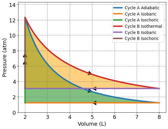
../../_images/0a21cc1e502f335558cb4ddfb2ac4a0cd1b5438be587b84261df762b98aef427.png

To compare the extracted work, we need to set up an equation that relates work to difference in volume and the starting point. In this example, each cycle begins at the same starting point and has the same change in volume. We will derive work equations for each process in terms of \(V_i\) and \(V_f\).

4.3.5.5.1. Work for Cycle A#

The work from Cycle A comes from the adiabat (\(w_A\)) and the isobaric process (\(w_I\)). There is no work extracted from the isochoric process. We will manipulate the work equation for each separately then add them together to have an equation that represents work for Cycle A. The equation we used to solve for work earlier on an adiabat is:

(4.227)#\[\begin{align} w_A &= \frac{3}{2}nR(T_f-T_i)\\ \end{align}\]

We will use the adiabat relationship \(TV^\frac{2}{3}\) to relate work to volume, not the temperature.

(4.228)#\[\begin{align} T_iV_i^\frac{2}{3} &= T_fV_f^\frac{2}{3} \\ \Rightarrow T_f &= T_i\cdot\left(\frac{V_i}{V_f}\right)^\frac{2}{3} \\ \end{align}\]

Substract \(T_i\) from each side substitutue into the work equation.

(4.229)#\[\begin{align} T_f -T_i &= T_i\cdot\left(\frac{V_i}{V_f}\right)^\frac{2}{3} -T_i \\ \Rightarrow w_A &= \frac{3}{2}nRT_i\cdot\left(\frac{V_i}{V_f}\right)^\frac{2}{3} -T_i \end{align}\]

We also need to work extracted from the isobaric process. Work from an isobaric process is calculated from \(w = -P\Delta V\). We will need to define \(\Delta V\) in terms of the whole cycle and define \(P\). For an adiabat \(P\) will be determined by the relationship \(PV^{5/3}\)

(4.230)#\[\begin{align} P_iV_i^{5/3} &= P_fV_f^{5/3} \\ \Rightarrow P_f &= P_i\cdot\left(\frac{V_i}{V_f}\right)^\frac{5}{3} \\ \end{align}\]

Initial pressure is determined by the starting point. Since we are given starting point values for \(V\) and \(T\) we can solve for \(P\) using the ideal gas law and substitute this relationship.

(4.231)#\[\begin{align} P_i &= \frac{nRT}{V_i} \\ \Rightarrow w_I &= -\frac{nRT}{V_i}\cdot\left(\frac{V_i}{V_f}\right)^\frac{5}{3}\cdot\Delta V \\ \end{align}\]

Finally, \(\Delta V\) refers to the change in volume in the isobaric process. In the three-membered cycle used in this example, the final volume of the isobaric process is equal to the initial volume. We can substitute \(\Delta V = V_i - V_f\). The resulting equation for work from the isobaric process of Cycle A is

(4.232)#\[\begin{align} w_I &= -\frac{nRT}{V_i}\cdot\left(\frac{V_i}{V_f}\right)^\frac{5}{3}\cdot(V_i - V_f) \\ \end{align}\]

To get the total work from Cycle A we will simplify and sum \(w_A\) and \(w_I\)

(4.233)#\[\begin{align} w &= nRT_i\cdot\left[\frac{3}{2}\left(\frac{V_i}{V_f}\right)^\frac{2}{3}-\frac{3}{2} -\frac{V_i - V_f}{V_i}\cdot\left(\frac{V_i}{V_f}\right)^\frac{5}{3}\right] \\ &= nRT_i\cdot\left[\frac{5}{2}\left(\frac{V_i}{V_f}\right)^\frac{2}{3}-\frac{3}{2} - \left(\frac{V_i}{V_f}\right)^\frac{5}{3}\right] \end{align}\]

To prove this equation works, below is the calculation for Cycle A that we solved earlier. The values match.

-14.94526550773886

4.3.5.5.2. Work for Cycle B#

We will do the same for Cycle B. The equation we used for work on an isotherm, \(w = nRT\ln(\frac{V_i}{V_f})\). This relationship is already in terms of initial and final volume. We also need to rearrange the isobaric process like we did for Cycle A. Work from an isobaric process is calculated from \(w = -P\Delta V\). We can use the ideal gas law to substitute for \(P\).

(4.234)#\[\begin{align} P_f &= \frac{nRT}{V_f} \\ \Rightarrow w &= \frac{nRT}{V_f}\cdot(V_i - V_f) \end{align}\]

Just as before we will sum the two processes to get total extractable work for Cycle B.

(4.235)#\[\begin{align} w &= nRT\left[ln\left(\frac{V_i}{V_f}\right)-\frac{V_i-V_f}{V_f}\right] \\ &= nRT\left[ln\left(\frac{V_i}{V_f}\right)+1 - \frac{V_i}{V_f}\right] \end{align}\]

To prove this equation is valid, below is the calculation for Cycle B that we solved earlier.

# compute work for process A in units of nR
import numpy as np
def wB(Ti,Vi_Vf):
    return Ti*(np.log(Vi_Vf) + 1 - Vi_Vf)

print(wB(300,2/8)*0.08206)

-15.664294582049465

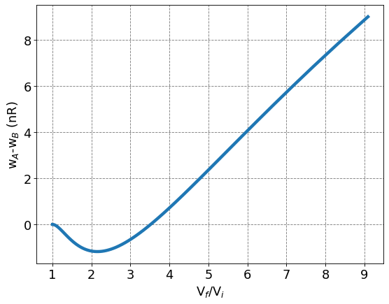
4.3.5.5.3. Ratio of extracted work from Cycle A or B based on change in volume#

Now that we have derived equations for work for each of these processes that are dependent on change in volume and starting at the same value, we can compare the work extracted from each process based on the ratio of volumes. The plot below shows that the difference in work extracted from Cycle A and Cycle B depends on the ratio between final and initial volume. If the ratio of final to initial volume is less than about 3.5, then Cycle B extracts more work than Cycle A.

import matplotlib.pyplot as plt
%matplotlib inline
# Plot
fontsize=16
fig, ax=plt.subplots(figsize=(8,6), dpi= 80, facecolor='w', edgecolor='k')
Ti = 300
Vi_Vf = np.arange(1,0.1,-0.01)
ax.plot(1/Vi_Vf, (wA(Ti,Vi_Vf) - wB(Ti,Vi_Vf))*0.08206, linewidth=4, label=r'w$_B$-w$_A$')
# Formatting
ax.set_xlabel(r'V$_f$/V$_i$', size=fontsize)
ax.set_ylabel(r'w$_A$-w$_B$ (nR)', size=fontsize)
ax.grid (which='major', axis='both', color='#808080', linestyle='--')
plt.tick_params(axis='both',labelsize=fontsize)

../../_images/63c262bf737202cbd4680e50f3d0788aa52cf53e6be59a2564ffe240308bd8bb.png

4.3.5.6. Summary#

To solve thermodyanamic problems on an exam, take advantage of relationships to minimize the number of calculations you need to set up. We solved for values on two different cycles. Work extracted depends on the starting point, ratio of volumes, and processes within the cycle.