Transition State Theory and Temperature Dependence of the Rate Constant

4.4.4. Transition State Theory and Temperature Dependence of the Rate Constant#

4.4.4.1. Motivation#

In these notes we will start to investigate some of the quantities that affect the rate constant. We will start by deriving the Transition State Theory version of the rate constant and then look at how this equation depends on temperature.

4.4.4.2. Learning Goals#

After working through these notes, you should be able to:

Derive Transition State Theory expressions for the rate constant
Describe how a rate constant depends on temperature
Identify the correspondence between activation energy and the TST rate constant expression
Compute the activation energy for a reaction from rate constant vs temperature data
Compute the Arhenius prefactor from rate constant vs temperature data

4.4.4.3. Coding Concepts#

The following coding concepts are used in this notebook:

4.4.4.4. Transition State Theory Expression for the Rate Constant#

So far we have more or less ignored the rate constants and yet the values of these constants has a dramatic effect on the rate of reaction. What are the molecular origins oof these values and why are some reactions faster than others?

Transition State Theory, first developed by Henry Eyring in the early 20th century, provides a model for the rate constant that matches experimental data. This result provides us with some insight into why certain reaction are faster than others.

For this derivation we consider a generic reaction

(4.539)#\[\begin{equation} A + B \rightarrow P \end{equation}\]

where the rate law is given as

(4.540)#\[\begin{equation} \frac{d[P]}{dt} = k[A][B] \end{equation}\]

Transition State Theory postulates the existence of an activated complex (or transition state species) that must be populated before the product is formed. That is, \(A\) and \(B\) are in an initial equilibrium with a high energy intermediate, or transition state, before forming the product, \(P\). The proposed mechanism is written as

(4.541)#\[\begin{equation} A + B \overset{k_1}{\underset{k_{-1}}{\rightleftharpoons}} AB^{\ddagger} \overset{k_2}{\rightarrow} P \end{equation}\]

The species \(AB^\ddagger\) denotes the transition state and is a considered the molecular “species” at the saddle point in the free energy surface between reactants and products. The initial equilibrium has equilibrium constant

(4.542)#\[\begin{equation} K_C^\ddagger = \frac{[AB^\ddagger]c^\circ}{[A][B]} \end{equation}\]

The rate of product formation, under the current proposed mechanism, is

(4.543)#\[\begin{equation} \frac{d[P]}{dt} = k_2[AB^\ddagger] \end{equation}\]

When developing rate laws from mechanisms, we avoid writing the overall rate law in terms of intermediates. Thus, we replace \([AB^\ddagger]\) with the equilibrium constant expression above to get

(4.544)#\[\begin{equation} \frac{d[P]}{dt} = k_2K_C^\ddagger(c^\circ)^{-1}[A][B] \end{equation}\]

If we compare this to the overall rate law we see that or TST mechanism suggests that

(4.545)#\[\begin{equation} k = k_2K_C^\ddagger(c^\circ)^{-1} \end{equation}\]

To further investigate the physical underpinnings of \(k_2\) and \(K_C^\ddagger\) we will use aspects of Statistical Thermodynamics. First, we recognize that \(k_2\) is related to the frequency of motion along the reaction coordinate (rc), \(\nu_{rc}\):

(4.546)#\[\begin{equation} k_2 = \nu_{rc} \end{equation}\]

Sometimes it is stated that \(k_2 = \kappa \nu_{rc}\) where \(\kappa\) is the transmission coefficient that dictates the fraction of vibrations in this direction that lead to product formation. Here will will simply use that \(\kappa = 1\).

Second, we will express the equilibrium constant in terms of partition functions

(4.547)#\[\begin{eqnarray} K_C^\ddagger = \frac{\left(\frac{q_{AB^\ddagger}}{V}\right)c^\circ}{\left(\frac{q_{A}}{V}\right)\left(\frac{q_{B}}{V}\right)} \end{eqnarray}\]

we will then extract from \(q_{AB^\ddagger}\) the motion along the reaction coordinate. That is we will dictate that \(q_{AB^\ddagger} = q_{rc}q_{int}\) yielding

(4.548)#\[\begin{eqnarray} K_C^\ddagger = q_{rc}\frac{\left(\frac{q_{int}}{V}\right)c^\circ}{\left(\frac{q_{A}}{V}\right)\left(\frac{q_{B}}{V}\right)} = q_{rc} K_C^{\ddagger*} \end{eqnarray}\]

where \(K_C^{\ddagger*}\) is the equilibrium constant between TS and reactants with the 1D motion along the reaction coordinate of the TS removed. It can be shown that

(4.549)#\[\begin{equation} \nu_{rc}q_{rc} = \frac{k_BT}{h} \end{equation}\]

Thus yielding

(4.550)#\[\begin{equation} k_{TST} = \frac{k_BT}{h}K_C^{\ddagger*}(c^\circ)^{-1} \end{equation}\]

Recall that the equlibrium constant can be expressed as \(K^\ddagger = e^{-\Delta G^{\ddagger\circ}/RT}\) yielding

(4.551)#\[\begin{eqnarray} k &=& k_2e^{-\Delta G^{\ddagger\circ}RT} \\ &=& k_2e^{\Delta S^{\ddagger\circ}/R}e^{-\Delta H^{\ddagger\circ}/RT} \end{eqnarray}\]

\(k_2\), the rate constant of the second step in the TST mechanism, is related to the frequency that the complexes cross over the barrier. It can be shown that, under consideration of one dimensional motion at the TS, that

(4.552)#\[\begin{equation} k_2 = \frac{k_BT}{hc^\circ} \end{equation}\]

Thus yielding the final expression for the TST rate constant of

(4.553)#\[\begin{equation} k = \frac{k_BT}{hc^\circ}e^{\Delta S^{\ddagger\circ}/R}e^{-\Delta H^{\ddagger\circ}/RT} \end{equation}\]

This form of the TST rate constant expression is for a second order reaction. More generally, we can write

(4.554)#\[\begin{equation} k = \frac{k_BT}{h}(c^\circ)^{1-m}e^{\Delta S^{\ddagger\circ}/R}e^{-\Delta H^{\ddagger\circ}/RT}, \end{equation}\]

where \(m\) is the order of the reaction.

The TST expression for the rate constant indicates that the overall rate constant will increase with:

Increasing temperature
Decreasing \(\Delta H^\ddagger\)
Increasing \(\Delta S^\ddagger\).

\(\Delta H^\ddagger\) is related to the activation energy of the reaction and \(\Delta S^\ddagger\) is related to the relative disorder of the TS and reactants.

4.4.4.5. The Temperature Depedence of the Rate Constant#

4.4.4.5.1. Arhenius Expression#

A simpler expression for the rate constant come from Arhenius. He expressed the rate constant as

(4.555)#\[\begin{equation} k = Ae^{-\frac{E_a}{RT}} \end{equation}\]

where \(A\) is the Arhenius prefactor and assumed to be temperature independent and \(E_a\) is the activation energy of the reaction. The linear form of the Arhenius equation is

(4.556)#\[\begin{equation} \ln k = -\frac{E_a}{RT} + \ln A. \end{equation}\]

This expression demonstrates that the log of a rate constant following the Arhenius expression will be linear with respect to \(1/T\).

Arhenius plots can be used to estimate the activation energy for a reaction.

4.4.4.5.2. Example: Activation Energy from Arhenius Plot#

The rate constant for the first order reaction

(4.557)#\[\begin{equation} N_2O_5(g) \rightarrow 2NO_2(g) + \frac{1}{2}O_2(g) \end{equation}\]

is measured as a function of temperature. From the table blelow determine the activation and Arhenius prexponential factor assuming Arhenius behavior.

T/K	273	298	308	318	328	338
k/\(10^{-5}\) s\(^{-1}\)	0.0787	3.46	13.5	49.8	150	487

To determine the activation energy, \(E_a\), and the Arhenius prefactor, \(A\), we will fit the following linear equation

(4.558)#\[\begin{equation} \ln k = -\frac{E_a}{RT} + \ln A. \end{equation}\]

To do so, we will plot \(\ln k\) vs \(1/T\)

import numpy as np
T = np.array([273, 298, 308, 318, 328, 338])
k = np.array([0.0787,3.46,13.5,49.8,150,487])*1e-5
print("1/T:", 1/T)
print("ln(k):",np.log(k))

1/T: [0.003663   0.0033557  0.00324675 0.00314465 0.00304878 0.00295858]
ln(k): [-14.05503759 -10.27165688  -8.91023578  -7.60491048  -6.50229017
  -5.32466134]

../../_images/f147032ce52f204d1d00cca6cb54bd496e39a41e3b0234b830e96011eba42e51.png

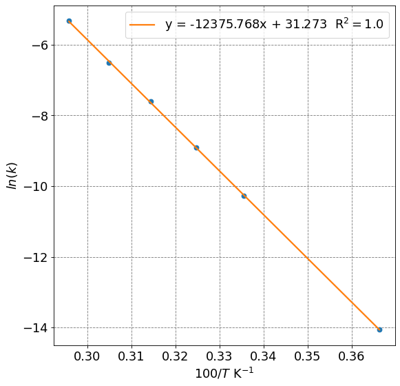
print("Activation energy:", np.round(-reg.coef_[0]*8.314/1000,0), "kJ/mol")
print("Prefactor:", np.exp(reg.intercept_), "1/s")

Activation energy: 103.0 kJ/mol
Prefactor: 38163368393980.85 1/s

From the fit to the line we have that

(4.559)#\[\begin{eqnarray} \text{slope} = -12375.768 &=& -\frac{E_a}{R} \\ \Rightarrow E_a &=& 12375.768\cdot R = 103 \text{ kJ}\cdot\text{mol}^{-1} \end{eqnarray}\]

and

(4.560)#\[\begin{eqnarray} \text{intercept} = 31.273 &=& \ln A \\ \Rightarrow A &=& e^{31.273} = 3.82\times10^{13} \text{ s}^{-1} \end{eqnarray}\]

4.4.4.5.3. TST and Arhenius#

The TST expression for the rate constant demonstrates a temperature dependence of both the exponential term and the prefactor. To demonstrate this we must start with a definition of activation energy from the Arhenius equation. That is

(4.561)#\[\begin{equation} E_a = RT^2\frac{d\ln k}{dT} \end{equation}\]

Now let’s determine \(\frac{d\ln k_{TST}}{dT}\)

(4.562)#\[\begin{eqnarray} \ln k_{TST} &=& \ln T - \frac{\Delta H^{\ddagger\circ}}{RT} + \ln\frac{k_B}{hc^\circ} + \frac{\Delta S^{\ddagger\circ}}{R} \\ \Rightarrow \frac{d \ln k_{TST}}{dT} &=& \frac{1}{T} + \frac{\Delta H^{\ddagger\circ}}{RT^2} \\ \Rightarrow E_{a,TST} &=& RT + \Delta H^{\ddagger\circ} \end{eqnarray}\]

By analogy we can also say that

(4.563)#\[\begin{equation} A_{TST} = \frac{k_BT}{h}(c^\circ)^{1-m}e^{\Delta S^{\ddagger\circ}/R} \end{equation}\]