4.5.14. Special Functions in Quantum Mechanics

4.5.14.1. Motivation:

We have encountered a number of new and named functions in this class so far. This has cause some confusion that I hope to alleviate with these notes.

4.5.14.2. Learning Goals:

After working through these notes, you will be able to:

1. Identify and use the Associated Legendre Polynomials

2. Employ the orthogonality relation of the Associated Legendre Polynomials

3. Identify where Associated Legendre Polynomials show up in QM

4. Identify and us the Spherical Bessel Functions

5. Employ the orthogonality relation of the Spherical Bessel Functions

6. Identify where Spherical Bessel Functions show up in QM

7. Identify and use the Associated Laguerre Polynomials

8. Identify where the Associated Laguerre Polynomials show up in QM

4.5.14.3. Coding Concepts:

The following coding concepts are used in this notebook:

1. Variables

2. Functions

3. Plotting with matplotlib

4.5.14.4. Associated Legendre Polynomials

The Associated Legendre Polynomials show up as the solution to the differential equation stemming from the \(\theta\) component of the Laplacian in spherical polar coordinates. After solving for the \(\phi\) component we end up with the equation

(4.878)\[\begin{equation} m^2 = \frac{\sin\theta}{\Theta(\theta)}\frac{\partial}{\partial\theta}\left(\sin\theta\frac{\partial}{\partial\theta}\right)\Theta(\theta)+\beta\sin^2\theta, \end{equation}\]

where \(m=0,\pm 1, \pm 2, ... \) from the periodicity of \(\phi\). Now make a change of variable \(x = \cos\theta\) which yields \(\frac{dx}{-\sin\theta}=d\theta\) and define \(P(x) = \Theta(\theta)\). Plugging these in and performing some rearrangements yields a differential equation that matches the general Legendre equation

(4.879)\[\begin{equation} (1-x^2)\frac{d^2P(x)}{dx^2}-2x\frac{dP(x)}{dx}+\left[\beta-\frac{m^2}{1-x^2}\right]P(x) = 0 \end{equation}\]

It turns out that for \(\Theta(\theta)\) to be continous \(\beta=l(l+1)\) where \(l=0,1,2...\). Note that this also puts a limit on \(m\) with \(m=0,1, 2, ... , l\).

The solutions, \(P_l^m(x)\), to the above equation are known as the Associated Legendre Polynomials. The specific functional form of these functions depends on both indeces \(m\) and \(l\). Index \(l\) is referred to as the degree and \(m\) is referred to as the order of the Associated Legendre Polynomial. The functions can be determined in a number of ways. A recursive formula for these functions is:

(4.880)\[\begin{equation} P_l^m(x) = (-1)^m(1-x^2)^{m/2}\frac{d^m}{dx^m}P_l(x), \end{equation}\]

where \(P_l(x)\) are the Legendre polynomials. The Legendre polynomials are solutions to the Legendre equation which differs from the general Legendre equation by the exclusion of the \(-\frac{m^2}{1-x^2}\) term.

In order to use the above equation to determine a specific functional form for the Associated Legendre Polynomials you need to know the target \(m\) and \(l\) as well as the Legendre polynomial \(P_l(x)\). There are a number of ways of defining these functions but perhaps the easiest way is the Rodriguez formula:

(4.881)\[\begin{equation} P_l(x) = \frac{1}{2^ll!}\frac{d^l}{dx^l}\left(x^2-1\right)^l \end{equation}\]

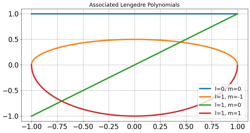
In general, however, it is easier to just look up the specific function. Below is a table of the first few Associated Lengedre polynomials followed by a plot of these functions

\(l\)	\(m\)	\(P_l^m(x)\)
0	0	\(P_0^0(x) = 1\)
\(1\)	\(-1\)	\(P_1^{-1}(x) = \frac{1}{2}\sqrt{1-x^2}\)
\(1\)	\(0\)	\(P_1^{0}(x) = x\)
\(1\)	\(1\)	\(P_1^{-1}(x) = -\sqrt{1-x^2}\)

Show code cell source Hide code cell source

# plot of some of the Legendre polynomials
import warnings
warnings.filterwarnings('ignore')
import numpy as np
import matplotlib.pyplot as plt
%matplotlib inline
from scipy.special import lpmv
x = np.arange(-1,1,0.0001)
plt.figure(figsize=(12,6),dpi= 80, facecolor='w', edgecolor='k')
plt.tick_params(axis='both',labelsize=20)
plt.grid(b=True, which='major', axis='both', color='#808080', linestyle='--')
for l in range(2):
    for m in range(-l,l+1):
        label = "l=" + str(l) + ", m=" + str(m)
        plt.plot(x,lpmv(m,l,x),lw=4,label=label)
plt.title("Associated Lengedre Polynomials",fontsize=16)
plt.legend(fontsize=16);

4.5.14.4.1. Orthogonality of the Associated Legendre Polynomials

The Associated Legendre Polynomials have the following orthogonality rules over the domain \(-1 \leq x \leq 1\):

(4.882)\[\begin{equation} \left\langle P_l^m|P_{l'}^m \right\rangle = \int_{-1}^{1} P_l^m(x)P_{l'}^m(x)dx = \frac{2(l+m)!}{(2l+1)(l-m)!}\delta_{l,l'} \end{equation}\]

That being that if \(m\) is kept constant, then an Associated Legendre Polynomial of one \(l\) value is orthogonal to an Associated Legendre Polynomial with a different \(l\) value. A more general orthogonality relationship does not exist. As you can see from the table below, certain pairs of Associated Legendre Polynomials are not orthogonal (e.g. \(P_0^0\) and \(P_1^1\)).

Show code cell source Hide code cell source

from scipy import integrate
from scipy.special import lpmv
import numpy as np
from scipy.special import factorial

def theta_norm(m,l):
    return np.sqrt(((2*l+1)*factorial(l-np.abs(m)))/(2*factorial(l+np.abs(m))))
def integrand(theta,m1,l1,m2,l2):
    return theta_norm(m1,l1)*lpmv(m1,l1,theta)*theta_norm(m2,l2)*lpmv(m2,l2,theta)

print ("{:<8} {:<8} {:<8} {:<8} {:<20}".format('l','m','l\'','m\'','<Theta_ml | Theta_m\'l\'>'))
print("-------------------------------------------------------------------------")
for l1 in range(3):
    for m1 in range(l1+1):
        for l2 in range(l1,3):
            for m2 in range(l2+1):
                print ("{:<8} {:<8} {:<8} {:<8} {:<20}".format(l1,m1,l2,m2,np.round(integrate.quad(integrand,-1,1,args=(m1,l1,m2,l2))[0],3)))

l        m        l'       m'       <Theta_ml | Theta_m'l'>
-------------------------------------------------------------------------
0        0        0        0        1.0                 
0        0        1        0        0.0                 
0        0        1        1        -0.962              
0        0        2        0        0.0                 
0        0        2        1        -0.0                
0        0        2        2        0.913               
1        0        1        0        1.0                 
1        0        1        1        0.0                 
1        0        2        0        0.0                 
1        0        2        1        -0.931              
1        0        2        2        -0.0                
1        1        1        0        -0.0                
1        1        1        1        1.0                 
1        1        2        0        0.269               
1        1        2        1        0.0                 
1        1        2        2        -0.988              
2        0        2        0        1.0                 
2        0        2        1        -0.0                
2        0        2        2        -0.408              
2        1        2        0        -0.0                
2        1        2        1        1.0                 
2        1        2        2        -0.0                
2        2        2        0        -0.408              
2        2        2        1        -0.0                
2        2        2        2        1.0                 

4.5.14.4.2. Use in Quantum Mechanics

The use of Associated Legendre Polynomials in quantum mechanics is obscured because of their inclusion in the spherical harmonics. These functions account for both the \(\theta\) and \(\phi\) components with the \(\theta\) component being the Associated Legendre Polynomials. The orthogonality of these functions combined with the \(\phi\) solutions is what yields the orthogonality of the spherical harmonics.

The normalized spherical harmonics are given by

(4.883)\[\begin{equation} Y_l^m = \sqrt{\frac{(2l+1)(l-|m|)!}{4\pi(l+|m|)!}}P_l^{|m|}(\cos\theta)e^{im\phi} \end{equation}\]

where \(P_l^{|m|}(\cos\theta)\) is the Associated Legendre Polynomial of degree \(l\) and order \(|m|\).

These functions do form a complete orthonormal basis for the space of \(\theta\) and \(\phi\). The orthonormality relationship for these functions is given as

(4.884)\[\begin{equation} \left\langle Y_l^m | Y_{l'}^{m'} \right\rangle = \delta_{l,l'}\delta_{m,m'} \end{equation}\]

Notice that the above orthogonality of the spherical harmonics and the lack of orthogonality of the Associated Legendre Polynomials when \(m\neq m'\) requires that the \(\phi\) component be orthogonal when \(m\neq m'\). We can demonstrate that with code (below) or simply recognize that

(4.885)\[\begin{equation} \int_0^{2\pi} e^{i(m-m')\phi}d\phi = 2\pi\delta_{m,m'} \end{equation}\]

Show code cell source Hide code cell source

from scipy import integrate
from scipy.special import lpmv
import numpy as np

def phi_norm2():
    return 1/(2*np.pi)
def real_integrand(phi,m1,m2):
    return phi_norm2()*np.cos((m1-m2)*phi)
def im_integrand(phi,m1,m2):
    return phi_norm2()*np.sin((m1-m2)*phi)

print ("{:<8} {:<8} {:<30} {:<30}".format('m','m\'','Re<Phi_m | Phi_m\'>','Im<Phi_m | Phi_m\'>'))
print("--------------------------------------------------------------------")
for m1 in range(4):
    for m2 in range(m1,4):
        print ("{:<8} {:<8} {:<30} {:<30}".format(m1,m2,np.round(integrate.quad(real_integrand,0,2*np.pi,args=(m1,m2))[0],3),np.round(integrate.quad(im_integrand,0,2*np.pi,args=(m1,m2))[0],3)))

m        m'       Re<Phi_m | Phi_m'>             Im<Phi_m | Phi_m'>            
--------------------------------------------------------------------
0        0        1.0                            0.0                           
0        1        0.0                            -0.0                          
0        2        -0.0                           0.0                           
0        3        -0.0                           -0.0                          
1        1        1.0                            0.0                           
1        2        0.0                            -0.0                          
1        3        -0.0                           0.0                           
2        2        1.0                            0.0                           
2        3        0.0                            -0.0                          
3        3        1.0                            0.0                           

4.5.14.5. Spherical Bessel Functions

The Spherical Bessel Functions show up as the solutions to the radial component of the particle in a sphere. In our solution for the radial component, \(r\), we started with an equation that resembled

(4.886)\[\begin{equation} \frac{\hbar^2}{R(r)}\frac{\partial}{\partial r}\left(r^2\frac{\partial}{\partial r}\right)R(r) + 2mr^2E = \hbar^2l(l+1) \end{equation}\]

where the \(l(l+1)\) part comes from the angular solutions. Rearranging yields

(4.887)\[\begin{equation} \frac{\partial}{\partial r}\left(r^2\frac{\partial}{\partial r}\right)R(r) + \left(\frac{2mE}{\hbar^2}r^2 - l(l+1)\right)R(r) = 0 \end{equation}\]

Now expanding the first term using the product rule we get

(4.888)\[\begin{align} &\left(r^2\frac{\partial^2R(r)}{\partial r^2} + 2r\frac{\partial R(r)}{\partial r}\right) + \left(\frac{2mE}{\hbar^2}r^2 - l(l+1)\right)R(r) = 0 \\ &r^2\frac{\partial^2R(r)}{\partial r^2} + 2r\frac{\partial R(r)}{\partial r} + \left(\frac{2mE}{\hbar^2}r^2 - l(l+1)\right)R(r) = 0 \end{align}\]

The above expression resembles a differential equation of the form

(4.889)\[\begin{equation} x^2\frac{d^2y(x)}{d x^2} + 2x\frac{d y(x)}{d x} + \left(x^2 - l(l+1)\right)y(x) = 0, \end{equation}\]

that has the spherical Bessel functions as the solutions. To get the final manipulation we must set \(x^2= \frac{2mE}{\hbar^2}r^2\) or \(x = \frac{\sqrt{2mE}}{\hbar}r\). Additionally, we introduce a new function \(y(x) = R(r)\) and recognize that

(4.890)\[\begin{align} \frac{d y(x)}{dx} &= \frac{dr}{dx}\frac{dR(r)}{dr} \\ \frac{d^2 y(x)}{dx^2} &= \frac{dr}{dx}\frac{dr}{dx}\frac{d^2R(r)}{dr^2} \end{align}\]

or

(4.891)\[\begin{align} \frac{dR(r)}{dr} &= \frac{dx}{dr}\frac{d y(x)}{dx} \\ \frac{d^2R(r)}{dr^2} &= \left(\frac{dx}{dr}\right)^2\frac{d^2 y(x)}{dx^2} \end{align}\]

Thus, we can see that our final radial differential equation will be exactly of the form for which the spherical Bessel functions are the solutions. Note, however, that the independent variable is actually \(x = \frac{\sqrt{2mE}}{\hbar}r\).

The spherical Bessel functions have two types. We will ignore the second type because it can be discarded as a solution to our problem due to postulate 1 of quantum mechanics (the function is not finite in the domain). The spherical Bessel functions of the first type are denoted \(j_l(x)\) as the specific functional form of these depends on the index \(l\). These functions are related to the ordinary Bessel functions of the first type, \(J_l(x)\), by the following relationship

(4.892)\[\begin{equation} j_l(x) = \sqrt{\frac{\pi}{2x}}J_{l+\frac{1}{2}}(x) \end{equation}\]

The spherical Bessel functions can also be determined using Rayleigh’s formula for them:

(4.893)\[\begin{equation} j_l(x) = (-x)^l\left(\frac{1}{x}\frac{d}{dx}\right)^l\frac{\sin x}{x} \end{equation}\]

The above equation can be used to determine the spherical Bessel function of the first type for integer \(l\). It is likely easier, however, to look up a table of these such as the one given below

\(l\)	\(j_l(x)\)
0	\(j_0(x) = \frac{\sin x}{x}\)
\(1\)	\(j_1(x) = \frac{\sin x}{x^2} - \frac{\cos x}{x}\)
\(2\)	\(j_2(x) = \left(\frac{3}{x^2} - 1 \right)\frac{\sin x}{x} - \frac{3\cos x}{x^2}\)

Show code cell source Hide code cell source

#### import numpy as np
import matplotlib.pyplot as plt
%matplotlib inline
from scipy.special import spherical_jn, spherical_yn
fontsize = 20
x = np.arange(0.0, 10.0, 0.01)
fig, ax = plt.subplots(1,2,figsize=(20,8),dpi= 80, facecolor='w', edgecolor='k')
ax[0].set_ylim(-0.5, 1.1)
ax[0].set_title(r'$j_l$', fontsize=2*fontsize)
ax[0].set_xlabel(r'$x$',size=fontsize)
ax[0].set_ylabel(r'$j_l(x)$',size=fontsize)
ax[0].tick_params(axis='both',labelsize=fontsize)
for n in np.arange(0, 4):
    ax[0].plot(x, spherical_jn(n, x), lw = 3, label=rf'$l={n}$')
ax[0].grid(b=True, which='major', axis='both', color='#808080', linestyle='--')
ax[0].legend(loc='best',fontsize=fontsize)
# second type
ax[1].set_ylim(-1, 1)
ax[1].set_title(r'$y_l$',fontsize=2*fontsize)
for n in np.arange(0, 4):
    ax[1].plot(x, spherical_yn(n, x), lw = 3, label=rf'$l={n}$')
ax[1].set_xlabel(r'$x$',size=fontsize)
ax[1].set_ylabel(r'$y_l(x)$',size=fontsize)
ax[1].tick_params(axis='both',labelsize=fontsize)
ax[1].legend(loc='best',fontsize=fontsize)
ax[1].grid(b=True, which='major', axis='both', color='#808080', linestyle='--')
plt.show();

---------------------------------------------------------------------------
NameError                                 Traceback (most recent call last)
/var/folders/td/dll8n_kj4vd0zxjm0xd9m7740000gq/T/ipykernel_24619/2310059482.py in <module>
      4 from scipy.special import spherical_jn, spherical_yn
      5 fontsize = 20
----> 6 x = np.arange(0.0, 10.0, 0.01)
      7 fig, ax = plt.subplots(1,2,figsize=(20,8),dpi= 80, facecolor='w', edgecolor='k')
      8 ax[0].set_ylim(-0.5, 1.1)

NameError: name 'np' is not defined

4.5.14.5.1. The Zeros of the Spherical Bessel Functions

The values of \(x\) for which

(4.894)\[\begin{equation} j_l(x) = 0 \end{equation}\]

are important for the problem of particle in a sphere because the boundary conditions of the problem dictate that

(4.895)\[\begin{equation} R(r_0) = 0 \end{equation}\]

for the sphere radius \(r_0\).

As may be evident in the plot above, each \(j_l(x)\) function will continue to oscillate as \(x\rightarrow\infty\). This means that there will be an infinite number of \(x\) positions at which \(j_l(x)=0\). We will denote these \(x\) values as \(\beta_{n,l}\), or the \(n\)th \(x\) value for which \(l\)th spherical Bessel function crosses zero. There is no easy way to determine these values for arbitrary \(l\) so we just tabulate them

l\n	1	2	3	4
0	\(\pi\)	\(2\pi\)	\(3\pi\)	\(4\pi\)
1	4.493	7.725	10.904	14.066
2	5.763	9.095	12.322	15.515

When we use these zeros and solve for the energy etc, we get that the radial wavefunction for the particle in a sphere has the form

(4.896)\[\begin{equation} R_{l,n}(r) = Aj_l\left(\frac{\beta_{n,l}}{r_0}r\right) \end{equation}\]

4.5.14.5.2. Orthogonality of the Spherical Bessel Functions

The spherical Bessel Functions, \(j_l\left(\frac{\beta_{n,l}r}{r_0}\right)\) are orthogonal for different \(n\) and constant \(l\) over the domain \(0 \leq r < r_0\). This orthonormality can be expressed as follows

(4.897)\[\begin{equation} \left\langle j_l\left(\frac{\beta_{n,l}}{r_0}r\right) | j_{l}\left(\frac{\beta_{n',l}}{r_0}r\right)\right\rangle = \int_0^{r_0} j_l\left(\frac{\beta_{n,l}}{r_0}r\right) j_{l}\left(\frac{\beta_{n',l}}{r_0}r\right) r^2dr = \frac{r_0^3\delta_{nn'}}{2}\left[ j_{l+1}(\beta_{n,l})\right] \end{equation}\]

Notice that this orthonormality is for the different zeros of the same spherical Bessel function. The orthogonality of different \(l\)s is not guaranteed.

Show code cell source Hide code cell source

import numpy as np
import matplotlib.pyplot as plt
from scipy.special import sph_harm
from scipy.special import spherical_jn
from scipy import integrate
%matplotlib inline
from scipy.optimize import root
    
def integrand(r,n1,l1,n2,l2):
    zero_l1n1 = spherical_jn_zero(l1, n1)
    zero_l2n2 = spherical_jn_zero(l2, n2)
    return r_norm(n1,l1)*spherical_jn(l1, r*zero_l1n1)*r_norm(n2,l2)*spherical_jn(l2, r*zero_l2n2)*r**2
def r_norm(n,l):
    zero_ln = spherical_jn_zero(l, n)
    return np.sqrt(2)/(spherical_jn(l+1, zero_ln))
    
    
def spherical_jn_zero(l, n, ngrid=100):
    """Returns nth zero of spherical bessel function of order l
    """
    if l > 0:
        # calculate on a sensible grid
        x = np.linspace(l, l + 2*n*(np.pi * (np.log(l)+1)), ngrid)
        y = spherical_jn(l, x)
    
        # Find m good initial guesses from where y switches sign
        diffs = np.sign(y)[1:] - np.sign(y)[:-1]
        ind0s = np.where(diffs)[0][:n]  # first m times sign of y changes
        x0s = x[ind0s]
    
        def fn(x):
            return spherical_jn(l, x)

        return [root(fn, x0).x[0] for x0 in x0s][-1]
    else:
        return n*np.pi
print ("{:<8} {:<8} {:<8} {:<8} {:<30}".format('n','l','n\'','l\'','<j_l(b_nl r) | j_l\'(b_n\'l\' r)>'))
print("--------------------------------------------------------------------")
for l1 in range(3):
    for n1 in range(1,4):
        for l2 in range(3):
            for n2 in range(1,4):
                print ("{:<8} {:<8} {:<8} {:<8} {:<30}".format(n1,l1,n2,l2,np.round(integrate.quad(integrand,0,1,args=(n1,l1,n2,l2))[0],3)))    

n        l        n'       l'       <j_l(b_nl r) | j_l'(b_n'l' r)>
--------------------------------------------------------------------
1        0        1        0        1.0                           
1        0        2        0        0.0                           
1        0        3        0        -0.0                          
1        0        1        1        0.959                         
1        0        2        1        -0.242                        
1        0        3        1        0.112                         
1        0        1        2        0.89                          
1        0        2        2        -0.368                        
1        0        3        2        0.196                         
2        0        1        0        0.0                           
2        0        2        0        1.0                           
2        0        3        0        0.0                           
2        0        1        1        0.279                         
2        0        2        1        0.895                         
2        0        3        1        -0.281                        
2        0        1        2        0.455                         
2        0        2        2        0.708                         
2        0        3        2        -0.396                        
3        0        1        0        0.0                           
3        0        2        0        -0.0                          
3        0        3        0        1.0                           
3        0        1        1        -0.043                        
3        0        2        1        0.366                         
3        0        3        1        0.852                         
3        0        1        2        0.008                         
3        0        2        2        0.603                         
3        0        3        2        0.577                         
1        1        1        0        0.959                         
1        1        2        0        0.279                         
1        1        3        0        -0.043                        
1        1        1        1        1.0                           
1        1        2        1        -0.0                          
1        1        3        1        -0.0                          
1        1        1        2        0.981                         
1        1        2        2        -0.181                        
1        1        3        2        0.064                         
2        1        1        0        -0.242                        
2        1        2        0        0.895                         
2        1        3        0        0.366                         
2        1        1        1        -0.0                          
2        1        2        1        1.0                           
2        1        3        1        0.0                           
2        1        1        2        0.195                         
2        1        2        2        0.943                         
2        1        3        2        -0.239                        
3        1        1        0        0.112                         
3        1        2        0        -0.281                        
3        1        3        0        0.852                         
3        1        1        1        -0.0                          
3        1        2        1        0.0                           
3        1        3        1        1.0                           
3        1        1        2        -0.021                        
3        1        2        2        0.276                         
3        1        3        2        0.91                          
1        2        1        0        0.89                          
1        2        2        0        0.455                         
1        2        3        0        0.008                         
1        2        1        1        0.981                         
1        2        2        1        0.195                         
1        2        3        1        -0.021                        
1        2        1        2        1.0                           
1        2        2        2        0.0                           
1        2        3        2        -0.0                          
2        2        1        0        -0.368                        
2        2        2        0        0.708                         
2        2        3        0        0.603                         
2        2        1        1        -0.181                        
2        2        2        1        0.943                         
2        2        3        1        0.276                         
2        2        1        2        0.0                           
2        2        2        2        1.0                           
2        2        3        2        -0.0                          
3        2        1        0        0.196                         
3        2        2        0        -0.396                        
3        2        3        0        0.577                         
3        2        1        1        0.064                         
3        2        2        1        -0.239                        
3        2        3        1        0.91                          
3        2        1        2        -0.0                          
3        2        2        2        -0.0                          
3        2        3        2        1.0                           

def j1(x):
    return np.sin(x)/x**2 - np.cos(x)/x
def j2(x):
    return (3/x**2-1)*np.sin(x)/x - 3*np.cos(x)/x**2
def r_int(x):
    zero_41 = spherical_jn_zero(1, 4)
    norm = 2/j2(zero_41)**2
    return x**3*j1(zero_41*x)**2
def int1(x,beta):
    return np.sin(beta*x)**2/(beta**4*x)
def int2(x,beta):
    return x*np.cos(beta*x)**2/(beta**2)
def int3(x,beta):
    return 2*np.sin(beta*x)*np.cos(beta*x)/beta**3
print("int1:", integrate.quad(int1,0,1,args=(zero_41))[0])
print("int2:", integrate.quad(int2,0,1,args=(zero_41))[0])
print("int3:", integrate.quad(int3,0,1,args=(zero_41))[0])
print(2/(spherical_jn(2, zero_41)**2)*(integrate.quad(int1,0,1,args=(zero_41))[0] + integrate.quad(int2,0,1,args=(zero_41))[0] - integrate.quad(int3,0,1,args=(zero_41))[0]))
print(integrate.quad(r_int,0,1)[0])
print(2/(spherical_jn(2, zero_41)**2)*1.294e-3)

int1: 4.9911975147348385e-05
int2: 0.0012698875933548103
int3: 2.5415821093449187e-05
0.5147966377079543
0.0012943837474087094
0.51464401536846

def r_integrand(r,n,l):
    zero_ln = spherical_jn_zero(l, n)
    r_norm = 2/spherical_jn(l+1, zero_ln)**2
    return r_norm*spherical_jn(l, zero_ln*r)**2*r**3
print(integrate.quad(r_integrand,0,1,args=(4,1))[0])

0.5147966377079543

zero_41 = spherical_jn_zero(1, 4)
print(zero_41)
print("j_2(beta_41) = ", spherical_jn(2, zero_41))

14.066193912831473
j_2(beta_41) =  -0.07091345945046217

4.5.14.5.3. Use in Quantum Mechanics

The spherical Bessel functions are the solutions to the radial component of the particle in a sphere. The ordinary Bessel functions are the solutions to the radial component of the particle in a disc/circle. These functions show up in spherically symmetric bounded problems with no potential. We are unlikely to encounter them again in this class.

4.5.14.6. The Associated Laguerre Polynomials

The Associated Laguerre Polynomials are a component of the radial solution to the hydrogen atom Schrodinger equation. After solving the angular component, the following differential equation can be achieved

\(-\frac{\hbar^2}{2m_er^2}\frac{\partial}{\partial r}\left(r^2\frac{\partial}{\partial r}\right)R(r)+\left[\frac{\hbar^2l(l+1)}{2m_er^2} + V(r)-E\right]R(r) =0 \).

This can be solved using power series solutions to differential equations but we will not go through it. Instead we will present the energies and wavefunctions

\(E_n = - \frac{m_ee^4}{8\epsilon_0^2h^2n^2} = - \frac{e^2}{8\pi\epsilon_0a_0n^2}\)

for \(n=1,2,...\) and \(a_0 = \frac{\epsilon_0h^2}{\pi m_ee^2}\) is the Bohr radius. These are actually the same energies obtained from the Bohr model of the hydrogen atom. Also notice that the energies are independent of \(l\). It should be noted that \(n\geq l+1 \) or \(0 \leq l \leq n-1\) for \(n=1,2,..\).

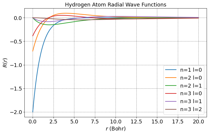
The radial wavefunction solution to the equation above is given as

\(R_{nl} = A_r r^le^{-r/na_0}L_{n+l}^{2l+1}\left( \frac{2r}{na_0}\right)\),

where \(L_{n+l}^{2l+1}\) are the associated Laguerre polynomials. Here is a table of the first few examples of these functions

\(n, l\)	\(L_{n+l}^{2l+1}(x)\)
\(1, 0\)	\(L_1^1(x)= -1\)
\(2, 0\)	\(L_2^1(x)= -2(2-x)\)
\(2, 1\)	\(L_3^3(x)= -3!\)
\(3, 0\)	\(L_3^1(x)= -3!(3-3x+\frac{1}{2}x^2)\)
\(3, 1\)	\(L_4^3(x)= -4!(4-x)\)
\(3, 2\)	\(L_5^5(x)= -5!\)

Show code cell source Hide code cell source

# let's plot some radial wavefunctions of the hydrogen atom
from scipy.special import sph_harm
from scipy.special import eval_genlaguerre
from scipy.special import factorial
from scipy import integrate
import numpy as np
import matplotlib.pyplot as plt
import warnings
warnings.filterwarnings('ignore')
%matplotlib inline
fontsize = 16
plt.figure(figsize=(10,6),dpi= 80, facecolor='w', edgecolor='k')
plt.tick_params(axis='both',labelsize=fontsize)
plt.grid(which='major', axis='both', color='#808080', linestyle='--')
plt.title("Hydrogen Atom Radial Wave Functions",fontsize=fontsize)
plt.legend(fontsize=fontsize);
# parameters for plotting
nLimit = 3
a0 = 1.0
r = np.arange(0,20,0.01)

for n in range(1,nLimit+1):
    for l in range(n):
        prefactor = -np.sqrt(factorial(n-l-1)/(2*n*factorial(n+l)))*(2.0/(n*a0))**(l+1.5)*np.power(r,l)*np.exp(-r/(n*a0))
        R = prefactor*eval_genlaguerre(n-l-1,2*l+1,2*r/(n*a0))
        label = "n=" + str(n) + " l=" + str(l)
        plt.plot(r,R,label=label,lw=2)
plt.legend(fontsize=fontsize)
plt.xlabel(r'$r$ (Bohr)',size=fontsize)
plt.ylabel(r'$R(r)$',size=fontsize)
plt.show();

No artists with labels found to put in legend.  Note that artists whose label start with an underscore are ignored when legend() is called with no argument.

4.5.14.6.1. Limited Orthogonality of the Laguerre Polynomials

The generalized Laguerre polynomials are not orthogonal themselves but are orthogonal over \([0,\infty)\) with weighting function \(x^\alpha e^{-x}\). That is

(4.898)\[\begin{equation} \int_0^\infty x^\alpha e^{-x} L_n^{(\alpha)}(x)L_m^{(\alpha)}(x)dx = \frac{\Gamma(n+\alpha+1)}{n!}\delta_{n,m} \end{equation}\]

where \(\Gamma\) is the gamma function and \(\delta_{n,m}\) is defined by

(4.899)\[\begin{equation} \delta_{n,m} = \begin{cases} 1 \quad\text{ if }n=m \\ 0 \quad\text{ otherwise}\end{cases} \end{equation}\]

That particular orthogonality condition is not that useful for us but it can also be shown that

(4.900)\[\begin{equation} \int_0^\infty x^{(\alpha+1)} e^{-x} L_n^{(\alpha)}(x)L_m^{(\alpha)}(x)dx = \frac{2n[(n+\frac{\alpha-1}{2})!]^3}{(n-\frac{(\alpha-1)}{2}-1)!}\delta_{n,m} \end{equation}\]

This relationship indicates that any two hydrogen atom wave functions differing in primary quantum number \(n\) and not \(l\) will be orthogonal. We will see that demonstrated in the table below

Show code cell source Hide code cell source

import numpy as np
from scipy import integrate
from scipy.special import eval_genlaguerre
from scipy.special import factorial
a0 = 1.0 # radial unit of Bohr!    
def hydrogen_atom_radial_wf(r,n,l):
    R_prefactor = -np.sqrt(factorial(n-l-1)/(2*n*factorial(n+l)))*(2.0/(n*a0))**(l+1.5)*np.power(r,l)*np.exp(-r/(n*a0))
    return R_prefactor*eval_genlaguerre(n-l-1,2*l+1,2*r/(n*a0))
def integrand(r,n1,l1,n2,l2):
    return r*r*hydrogen_atom_radial_wf(r,n1,l1)*hydrogen_atom_radial_wf(r,n2,l2)

print ("{:<10} {:<10} {:<10} {:<10} {:<20}".format('n', 'l', 'n\'', 'l\'', '<R_nl | R_n\'l\'>'))
print("--------------------------------------------------------------------")
for n1 in range(1,4):
    for l1 in range(n1):
        for n2 in range(1,4):
            for l2 in range(n2):
                print ("{:<10} {:<10} {:<10} {:<10} {:<20}".format(n1, l1, n2, l2, np.round(integrate.quad(integrand,0,np.infty,args=(n1,l1,n2,l2))[0],3)))

n          l          n'         l'         <R_nl | R_n'l'>     
--------------------------------------------------------------------
1          0          1          0          1.0                 
1          0          2          0          -0.0                
1          0          2          1          0.484               
1          0          3          0          -0.0                
1          0          3          1          0.23                
1          0          3          2          0.103               
2          0          1          0          -0.0                
2          0          2          0          1.0                 
2          0          2          1          -0.866              
2          0          3          0          0.0                 
2          0          3          1          0.213               
2          0          3          2          -0.761              
2          1          1          0          0.484               
2          1          2          0          -0.866              
2          1          2          1          1.0                 
2          1          3          0          -0.065              
2          1          3          1          0.0                 
2          1          3          2          0.659               
3          0          1          0          -0.0                
3          0          2          0          0.0                 
3          0          2          1          -0.065              
3          0          3          0          1.0                 
3          0          3          1          -0.943              
3          0          3          2          0.632               
3          1          1          0          0.23                
3          1          2          0          0.213               
3          1          2          1          0.0                 
3          1          3          0          -0.943              
3          1          3          1          1.0                 
3          1          3          2          -0.745              
3          2          1          0          0.103               
3          2          2          0          -0.761              
3          2          2          1          0.659               
3          2          3          0          0.632               
3          2          3          1          -0.745              
3          2          3          2          1.0                 

import numpy as np
import matplotlib.pyplot as plt
from scipy.special import sph_harm
from scipy.special import spherical_jn
from scipy import integrate
%matplotlib inline
from scipy.optimize import root
    
def integrand(r,n1,l1,n2,l2):
    zero_l1n1 = spherical_jn_zero(l1, n1)
    zero_l2n2 = spherical_jn_zero(l2, n2)
    return spherical_jn(l1, r*zero_l1n1)*spherical_jn(l2, r*zero_l2n2)*r**2
def integrand_norm(r,n1,l1,n2,l2):
    zero_l1n1 = spherical_jn_zero(l1, n1)
    zero_l2n2 = spherical_jn_zero(l2, n2)
    return r_norm(n1,l1)*r_norm(n2,l2)*spherical_jn(l1, r*zero_l1n1)*spherical_jn(l2, r*zero_l2n2)*r**2
def integrand_r3(r,n1,l1,n2,l2):
    zero_l1n1 = spherical_jn_zero(l1, n1)
    zero_l2n2 = spherical_jn_zero(l2, n2)
    return spherical_jn(l1, r*zero_l1n1)*spherical_jn(l2, r*zero_l2n2)*r**3
def r_norm(n,l):
    zero_ln = spherical_jn_zero(l, n)
    return np.sqrt(2)/(spherical_jn(l+1, zero_ln))
    
    
def spherical_jn_zero(l, n, ngrid=100):
    """Returns nth zero of spherical bessel function of order l
    """
    if l > 0:
        # calculate on a sensible grid
        x = np.linspace(l, l + 2*n*(np.pi * (np.log(l)+1)), ngrid)
        y = spherical_jn(l, x)
    
        # Find m good initial guesses from where y switches sign
        diffs = np.sign(y)[1:] - np.sign(y)[:-1]
        ind0s = np.where(diffs)[0][:n]  # first m times sign of y changes
        x0s = x[ind0s]
    
        def fn(x):
            return spherical_jn(l, x)

        return [root(fn, x0).x[0] for x0 in x0s][-1]
    else:
        return n*np.pi

print(np.round(integrate.quad(integrand_norm,0,1,args=(2,1,2,1))[0],10))
print(np.round(integrate.quad(integrand,0,1,args=(2,1,2,1))[0],10))
print(np.round(integrate.quad(integrand_r3,0,1,args=(2,1,2,1))[0],10))

1.0
0.008240013
0.0044444399

print(r_norm(2,1)**(2))
beta_21 = spherical_jn_zero(1,2)
print(spherical_jn(2,beta_21)**2)
print(2/spherical_jn(2,beta_21)**2)

121.35903188821808
0.01648002599297405
121.35903188821806

4.5.14.6.2. Use in Quantum Mechanics

The Associated Laguerre Polynomials show up in the radial solution to the hydrogen atom. They are a component of our understanding of radial wavefunctions for atoms and are thus extremely important. They may come up as basis functions in approximation methods for many electron atoms.