Second Law of Thermodynamics

4.3.8. Second Law of Thermodynamics#

import numpy as np
import matplotlib.pyplot as plt
%matplotlib inline
import plotting as myplt

---------------------------------------------------------------------------
ModuleNotFoundError                       Traceback (most recent call last)
/var/folders/td/dll8n_kj4vd0zxjm0xd9m7740000gq/T/ipykernel_33220/172206909.py in <module>
      2 import matplotlib.pyplot as plt
      3 get_ipython().run_line_magic('matplotlib', 'inline')
----> 4 import plotting as myplt

ModuleNotFoundError: No module named 'plotting'

Four equivalent statements of the 2nd Law:

Entropy is a state function that increases for all spontaneous processes (\(\Delta S_{univ} > 0\)). \(\Delta S = \int \frac{\delta q_{rev}}{T}\). The functin \(\frac{q}{T}\) is maximized for a reversible process.
Spontaneous changes are those from which work can be extracted. If done reversibly, the they yield a maximum amount of work.
Heat spontaneously flows from hot to cold and not in the reverse direction.
\(dS \geq \frac{\delta q}{T}\) where \(S\) is entropy and the equality holds for a reversible process.

4.3.8.1. Entropy is a State Function#

We will prove that an additional state function exists. We will call it entropy.

A state function other that internal energy and enthalpy must exist. The proof is as follows.

(4.268)#\[\begin{align} dU =& \delta q + \delta w \\ =& \delta q_{rev} - PdV \end{align}\]

where the last equality is for a reversible process for which there is only \(PV\) work. Since the left-hand side of this equation is the differential of a state function (\(dU\)), we are free to follow any desired path. We now, however, dictate that the system is an ideal gas meaning \(dU = C_VdT\) and \(P=\frac{nRT}{B}\):

(4.269)#\[\begin{align} dU =& C_VdT = \delta q_{rev} - \frac{nRT}{V}dV \\ \Rightarrow \delta q_{rev} =& C_VdT + \frac{nRT}{V}dV \end{align}\]

where I have solved the top equation for \(\delta q_{rev}\) to achieve the bottom equation. Now I will divide this bottom equation by \(T\) to achieve a separation of variables:

(4.270)#\[\begin{align} \frac{\delta q_{rev}}{T} =& \frac{C_V}{T}dT + \frac{nR}{V}dV \end{align}\]

Integrating both sides of this equation yields

(4.271)#\[\begin{align} \int\frac{\delta q_{rev}}{T} =& \int_{T_1}^{T_2}\frac{C_V}{T}dT + \int_{V_1}^{V_2}\frac{nR}{V}dV \\ =& C_V\ln\left(\frac{T_2}{T_1}\right) + nR\ln\left( \frac{V_2}{V_1} \right) \end{align}\]

We note that the right hand side (rhs) of this equation is a state function. This can be inferred because it only depends on the final state (\(V_2\) and \(T_2\)) and initial state (\(V_1\) and \(T_1\)). Since the rhs of the equaution is a state function, the lhs of the equation must also be a state function. We call this the change in entropy:

(4.272)#\[\begin{equation} \Delta S = \int\frac{\delta q_{rev}}{T} \end{equation}\]

or

(4.273)#\[\begin{equation} d S = \frac{\delta q_{rev}}{T} \end{equation}\]

4.3.8.2. Example#

Let’s consider an expansion/contraction of an ideal gas and compute the heat and entropy along two different paths

Compute \(q_{sys}\) and \(\Delta S_{sys}\) for the isothermal expansion of a gas from \(V_1\) to \(V_2=2V_1\) if done:

(a) Reversibly

(b) Against constant external pressure \(P_{ext} = P_2\)

(a) Reversible isothermal expansion from \(V_1\) to \(V_2=2V_1\):

Start by computing \(q_{sys}\):

(4.274)#\[\begin{align} q_{sys}^{(a)} = &nRT\ln\left(\frac{V_2}{V_1}\right)\\ = & nRT\ln\left(\frac{2V_1}{V_1}\right)\\ = & nRT\ln2 \end{align}\]

Note that \(q_{sys}^{(a)}>0\) meaning that the surroundings are providing heat to the system to cause this expansion.

Now \(\Delta S\)

(4.275)#\[\begin{align} \Delta S_{sys} = & \frac{\delta q_{rev}}{T} \\ = & \frac{nRT\ln2}{T} \\ = & nR\ln2 \end{align}\]

(b) Expansion from \(V_1\) to \(V_2\) against constant external pressure \(P_{ext} = P_2\)

Again, we start by computing \(q_{sys}^{(b)}\):

(4.276)#\[\begin{align} \Delta U_sys &= 0 = q_{sys}^{(b)} + w_{sys}^{(b)} \\ \Rightarrow q_{sys}^{(b)} &= - w_{sys}^{(b)} \\ &= P_2\Delta V \\ \end{align}\]

Now plug in \(P_2 = \frac{nRT}{V_2}\) and \(\Delta V = V_2 - V_1 = \frac{1}{2}V_2\):

(4.277)#\[\begin{align} q_{sys}^{(b)} &= P_2\Delta V \\ &= \frac{nRT}{V_2}\frac{V_2}{2} \\ &= \frac{nRT}{2} \\ \end{align}\]

Since entropy is a state function we still have:

(4.278)#\[\begin{align} \Delta S_{sys} = nR\ln2 \end{align}\]

Compare part (a) and part (b):

Entropies are identical since entropy is a state function.

Heat:

(4.279)#\[\begin{align} q_{sys}^{(a)} = & nRT\ln2 \\ q_{sys}^{(b)} =& \frac{nRT}{2} \end{align}\]

Which is bigger?

(4.280)#\[\begin{align} \frac{q_{sys}^{(a)}}{q_{sys}^{(b)}} = & \frac{nRT\ln2}{\frac{nRT}{2}} \\ =& 2\ln2 \\ \approx & 1.386 > 1 \end{align}\]

Thus we see that \(q\) is larger for the reversible process (a) than the irreversible process (b). Equivalently, \(-w\), the extractable work, is maximized in process (a).

4.3.8.3. Carnot Cycle (again)#

Compute the change in entropy (\(\Delta S\)) for each step along the Carnot cycle and show that \(\Delta S_{total} = 0\).

def plot_PV_diagram_adiabat(n=1,R=0.08206,V=np.arange(0.5,7.1,0.1),pUnit="atm",vUnit="L",T1=100,T2=200):
    xlabel = "V (" + vUnit + ")"
    ylabel = "P (" + pUnit + ")"
    fig, ax = myplt.define_figure(xlabel=xlabel,ylabel=ylabel)
    label = "T$_1$=" + str(T1)+" K"
    ax.plot(V,n*R*T1/V,label=label,lw=4)
    label = "T$_2$=" + str(T2)+" K"
    ax.plot(V,n*R*T2/V,label=label,lw=4)
    # adiabat 1
    lowV = (T1*1.5**(2/3)/T2)**(3/2)
    highV = 1.5
    Vadiabat1 = np.arange(lowV,highV+0.1,0.1)
    ax.plot(V,n*R*T1*1.5**(2/3)/V**(5/3),label="Adiabat 1",lw=4)
    ax.plot(Vadiabat1,n*R*T1*1.5**(2/3)/Vadiabat1**(5/3),lw=1,c="k")
    label = "(" + str(1.5) +","+ str(np.round(n*R*T1/1.5,decimals=1)) + "," +str(T1)+")"
    label = "(V$_1$,P$_1$,T$_1$)"
    ax.annotate(label,xy=(0.5,n*R*T1/1.5-1),fontsize=16)
    plt.scatter(1.5,n*R*T1/1.5,s=50,color="tab:blue")
    label = "(" + str(1.5) +","+ str(np.round(n*R*T2/1.5,decimals=1)) + "," +str(T2)+")"
    label = "(V$_2$,P$_2$,T$_2$)"
    plt.scatter(lowV,n*R*T2/lowV,s=50,color="tab:orange")
    ax.annotate(label,xy=(lowV+0.05,n*R*T2/lowV),fontsize=16)
    ax.annotate("A",xy=(0.4,n*R*T1/1.5+ 0.5*(n*R*T2/lowV-n*R*T1/1.5)),fontsize=24)
    label = "(" + str(2.5) +","+ str(np.round(n*R*T2/2.5,decimals=1)) + "," +str(T2)+")"
    label = "(V$_3$,P$_3$,T$_2$)"
    # adiabat 2
    lowV2 = 2.5
    highV2 = (T2*2.5**(2/3)/T1)**(3/2)
    Vadiabat2 = np.arange(lowV2,highV2+0.1,0.1)
    ax.plot(V,n*R*T2*2.5**(2/3)/V**(5/3),label="Adiabat 2",lw=4)
    ax.plot(Vadiabat2,n*R*T2*2.5**(2/3)/Vadiabat2**(5/3),lw=1,c="k")
    plt.scatter(2.5,n*R*T2/2.5,s=50,color="tab:orange")
    ax.annotate(label,xy=(2.6,n*R*T2/2.5),fontsize=16)
    ax.annotate("B",xy=(1.5,n*R*T2/2+3),fontsize=24)
    label = "(" + str(2.5) +","+ str(np.round(n*R*T1/2.5,decimals=1)) + "," +str(T1)+")"
    label = "(V$_4$,P$_4$,T$_1$)"
    plt.scatter(highV2,n*R*T1/highV2,s=50,color="tab:blue")
    ax.annotate(label,xy=(highV2,n*R*T1/highV2),fontsize=16)
    ax.annotate("C",xy=(4.25,3.0),fontsize=24)
    ax.annotate("D",xy=(3,n*R*T1/2-3.0),fontsize=24)
    #ax.annotate('',xytext=(1.5,n*R*T1/1.5),xy=(1.5,n*R*T2/1.5),arrowprops={'arrowstyle':"-",'lw': 2, 'color': 'black'})
    #ax.annotate('',xytext=(2.5,n*R*T1/2.5),xy=(2.5,n*R*T2/2.5),arrowprops={'arrowstyle':"-",'lw': 2, 'color': 'black'})
    #ax.annotate('',xy=(2.5,5.0),xytext=(2.5,5.1),arrowprops={'arrowstyle': 'simple','lw': 2, 'color': 'black'})
    #ax.annotate('',xy=(1.5,8.2),xytext=(1.5,8.1),arrowprops={'arrowstyle': 'simple','lw': 2, 'color': 'black'})
    vsub = np.arange(lowV,2.51,0.01)
    ax.plot(vsub,n*R*T2/vsub,lw=1,c="k")
    vsub = np.arange(1.5,highV2+0.01,0.01)
    ax.plot(vsub,n*R*T1/vsub,lw=1,c="k")
    ax.fill_between(np.arange(1.5,2.51,0.01),n*R*T1/np.arange(1.5,2.51,0.01),n*R*T2/np.arange(1.5,2.51,0.01),facecolor="purple",alpha=0.5,interpolate=True)
    ax.fill_between(np.arange(lowV,1.51,0.01),n*R*T2/np.arange(lowV,1.51,0.01),n*R*T1*1.5**(2/3)/np.arange(lowV,1.51,0.01)**(5/3),facecolor="purple",alpha=0.5,interpolate=True)
    ax.fill_between(np.arange(2.5,highV2+0.01,0.01),n*R*T2*2.5**(2/3)/np.arange(2.5,highV2+0.01,0.01)**(5/3),n*R*T1/np.arange(2.5,highV2+0.01,0.01),facecolor="purple",alpha=0.5,interpolate=True)
    ax.set_ylim(0,35)
    plt.legend(fontsize=16)

plot_PV_diagram_adiabat()

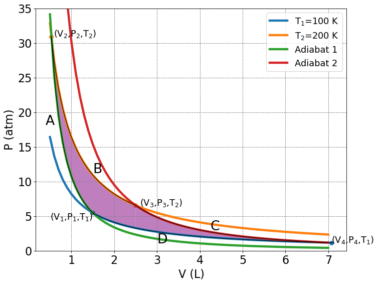
../../_images/86b90a4ab5bf92e97b7bc99b329026e651f6b0c750a3d8ae01979fb2ef7a2df3.png

4.3.8.3.1. \(A\) : Reversible Adiabatic Contraction#

Since the process is reversible and \(q_A = 0\), we have

(4.281)#\[\begin{equation} \Delta S_A = 0 \end{equation}\]

4.3.8.3.2. \(B\) : Reversible Isothermal Expansion#

Since the process is reversible and \(q_B = nRT_2\ln\left(\frac{V_3}{V_2}\right)\), we have

(4.282)#\[\begin{align} \Delta S_B &= \frac{q_{B,rev}}{T_B} \\ &= \frac{nRT_2\ln\left(\frac{V_3}{V_2}\right)}{T_2} \\ &= nR\ln\left(\frac{V_3}{V_2}\right) \end{align}\]

4.3.8.3.3. \(C\) : Reversible Adiabatic Expansion#

Since the process is reversible and \(q_C = 0\), we have

(4.283)#\[\begin{equation} \Delta S_C = 0 \end{equation}\]

4.3.8.3.4. \(D\) : Reversible Isothermal Contraction#

Since the process is reversible and \(q_D = nRT_1\ln\left(\frac{V_1}{V_4}\right)\), we have

(4.284)#\[\begin{align} \Delta S_D &= \frac{q_{D,rev}}{T_D} \\ &= \frac{nRT_1\ln\left(\frac{V_1}{V_4}\right)}{T_1} \\ &= nR\ln\left(\frac{V_1}{V_4}\right) \end{align}\]

4.3.8.3.5. Summary#

Process	\(w\)	\(q\)	\(\Delta U\)	\(\Delta H\)	\(\Delta S\)
A - Adiabatic Contraction	\(\frac{3}{2}nR(T_2-T_1)\)	\(0\)	\(\frac{3}{2}nR(T_2-T_1)\)	\(\frac{5}{2}nR(T_2-T_1)\)	\(0\)
B - Isothermal Expansion	\(nRT_2\ln\left(\frac{V_2}{V_3}\right)\)	\(nRT_2\ln\left(\frac{V_3}{V_2}\right)\)	\(0\)	\(0\)	\(nR\ln\left(\frac{V_3}{V_2}\right)\)
C - Adiabatic Expansion	\(\frac{3}{2}nR(T_1-T_2)\)	\(0\)	\(\frac{3}{2}nR(T_1-T_2)\)	\(\frac{5}{2}nR(T_1-T_2)\)	\(0\)
D - Isothermal Contraction	\(nRT_1\ln\left(\frac{V_4}{V_1}\right)\)	\(nRT_1\ln\left(\frac{V_1}{V_4}\right)\)	\(0\)	\(0\)	\(nR\ln\left(\frac{V_1}{V_4}\right)\)

4.3.8.3.6. Efficiency#

For a heat engine (\(w_{total}<0\)), the efficiency is the amount of work extracted, \(w_{total}\), divided by the energy in put, \(q_{in}\).

\(\varepsilon = \frac{w_{total}}{q_{in}}\)

For the Carnot cycle, this becomes:

\(\varepsilon = \frac{T_h-T_c}{T_h}\)