4.3.20. Chemical Equilibrium

4.3.20.1. Motivation

The application of Thermodynamics to chemical equilibrium is one of the most important outcomes in this class. We will like to not only predict whether a reaction happens but rather how much product is formed and how that varies with parameters such as temperature and pressure.

4.3.20.2. Learning Goals

After working through these notes, you will be able to:

1. Express the Gibbs free energy of a reaction in terms of the extent of reaction (\(\xi\))

2. Express the relationship between the standard Gibbs free energy of reaction and the equilibrium constant

3. Express the relationship between the Gibbs free energy of reaction and the reaction quotient

4. Use \(G(\xi)\) to determine \(\xi\) at equilibrium

5. Van’t Hoff

4.3.20.3. Coding Concepts

The following coding concepts are used in this notebook:

1. Variables

2. Functions

3. Plotting with matplotlib

4.3.20.4. Chemical Equilibrium

Here we consider chemical reactions such as

(4.463)\[\begin{equation} v_A A(g) + v_B B(g) \rightleftharpoons v_yY(g) + v_z Z(g) \end{equation}\]

We define a quantity, \(\xi\), called the extent of reaction, such that the number of moles of the reactants and products are given by

(4.464)\[\begin{eqnarray} n_A &=& n_{A0} - v_A\xi\\ n_B &=& n_{B0} - v_B\xi\\ n_Y &=& n_{Y0} + v_Y\xi\\ n_Z &=& n_{Z0} + v_Z\xi \end{eqnarray}\]

where \(n_{A0}\) is the initial number of moles of species \(A\).

If we take the differential of both sides we get

(4.465)\[\begin{eqnarray} dn_A &=& - v_Ad\xi\\ dn_B &=& - v_Bd\xi\\ dn_Y &=& v_Yd\xi\\ dn_Z &=& v_Zd\xi \end{eqnarray}\]

The differential of Gibbs free energy at constant \(T\) and \(P\) is

(4.466)\[\begin{eqnarray} dG &=& \mu_Adn_A + \mu_Bdn_B + \mu_Ydn_Y + \mu_Zdn_Z \\ &=& (-v_A\mu_A 0 v_B\mu_B + v_Y\mu_Y + v_Z\mu_Z)d\xi \\ \end{eqnarray}\]

or

(4.467)\[\begin{equation} \left( \frac{\partial G}{\partial \xi} \right)_{T,P} = (v_Y\mu_Y + v_Z\mu_Z - v_A\mu_A - v_B\mu_B) \end{equation}\]

The above equation is defined as the change in free energy of reaction, \(\Delta \bar{G}_{rxn}\).

If we assume each component acts as an ideal gas we get

(4.468)\[\begin{eqnarray} \Delta \bar{G}_{rxn} &=& v_Y\mu^\circ_Y(T) + v_Z\mu^\circ_Z(T)RT - v_A\mu^\circ_A(T) - v_B\mu^\circ_B(T) + \left( v_Y\ln\frac{P_Y}{P^0} + v_Z\ln\frac{P_Z}{P^0} - v_A\ln\frac{P_A}{P^0} - v_B\ln\frac{P_B}{P^0} \right) \\ &=& \Delta \bar{G}^0 + RT\ln Q \end{eqnarray}\]

At equilibrium we have that \(\Delta\bar{G}_{rxn}=0\) which yields

(4.469)\[\begin{equation} \Delta \bar{G}^0 = - RT\ln K_{eq} \end{equation}\]

4.3.20.5. dG = 0 at Equilibrium

Consider the example equilibrium maintained at 298.15 K and at 1 bar of pressure

(4.470)\[\begin{equation} N_2O_4(g) \rightleftharpoons 2NO_2(g) \end{equation}\]

If we start with 1 mole of reactants, we can write the extent of reaction as

(4.471)\[\begin{eqnarray} n_{N_2O_4} &=& 1 - \xi \\ n_{NO_2} &=& 2\xi \end{eqnarray}\]

This allows us to write the Gibbs energy as a function of \(\xi\):

(4.472)\[\begin{eqnarray} G &=& n_{N_2O_4}\bar{\mu}_{N_2O_4} + n_{NO_2}\bar{\mu}_{NO_2} \\ \Rightarrow G(\xi) &=& (1-\xi)\bar{\mu}_{N_2O_4} + 2\xi\bar{\mu}_{NO_2}\\ &=& (1-\xi)\left( \bar{\mu}^\circ_{N_2O_4} +RT\ln P_{N_2O_4}\right) + 2\xi\left( \bar{\mu}^\circ_{NO_2} +RT\ln P_{NO_2}\right) \\ &=& (1-\xi)\bar{\mu}^\circ_{N_2O_4} + 2\xi\bar{\mu}^\circ_{NO_2} + (1-\xi)RT\ln P_{N_2O_4} + 2\xi RT\ln P_{NO_2} \end{eqnarray}\]

where we have assumed that each gas is ideal.

Since the reaction is carred out a constant pressure of \(P=1\) bar and we have already assumed each gas is ideal, it follows that

(4.473)\[\begin{eqnarray} P_{N_2O_4} &=& x_{N_2O_4} \\ P_{NO_2} &=& x_{NO_2} \end{eqnarray}\]

The total number of moles is fixed so that we have

(4.474)\[\begin{eqnarray} P_{N_2O_4} &=& x_{N_2O_4} = \frac{1-\xi}{1+\xi} \\ P_{NO_2} &=& x_{NO_2} = \frac{2\xi}{1+\xi} \end{eqnarray}\]

Additionally, we will use that \(\bar{\mu}^\circ_{N_2O_4} = \Delta G^\circ_f = 97.787\) kJ\(\cdot\)mol\(^{-1}\) and \(\bar{\mu}^\circ_{NO_2} = \Delta G^\circ_f = 51.258\) kJ\(\cdot\)mol\(^{-1}\).

Plugging these into the equation for \(G(\xi)\) we get

(4.475)\[\begin{eqnarray} G(\xi) &=& (1-\xi)\Delta G^\circ_{f,N_2O_4} + 2\xi\Delta G^\circ_{f,NO_2} + (1-\xi)RT\ln \frac{1-\xi}{1+\xi} + 2\xi RT\ln \frac{2\xi}{1+\xi} \end{eqnarray}\]

This function is plotted below.

Show code cell source Hide code cell source

import numpy as np
print("∆G0_rxn = ", 2*51.258 - 97.87)
print("K_P = ", np.exp( -(2*51.258 - 97.787)/(8.314/1000*298.15)))

∆G0_rxn =  4.646000000000001
K_P =  0.14841197504828846

np.roots([4.14841197504828846,0,-0.14841197504828846])

array([-0.18914442,  0.18914442])

2*0.18914442/(1+0.18914442)

0.31811850069481046

from scipy.optimize import fsolve
f = lambda x: np.exp(-(2*51.258-97.787)/(8.314/1000*298.15))*(1-x) - 4*x**2
fsolve(f,[0.1,0.4])

array([0.17496117, 0.17496117])

print("Number of moles of NO2 at eq: ", 2*0.1776273)

Number of moles of NO2 at eq:  0.3552546

# define G function
import numpy as np
R = 8.314/1000
T = 298.15
def G(xi):
    return (1-xi)*97.87+2*xi*51.258 + (1-xi)*R*T*np.log((1-xi)/(1+xi)) + 2*xi*R*T*np.log(2*xi/(1+xi))

Show code cell source Hide code cell source

import matplotlib.pyplot as plt
%matplotlib inline
#define function 
# setup plot parameters
fontsize=16
fig = plt.figure(figsize=(8,8), dpi= 80, facecolor='w', edgecolor='k')
ax = plt.subplot(111)
ax.grid(which='major', axis='both', color='#808080', linestyle='--')
ax.set_xlabel("$xi$",size=fontsize)
ax.set_ylabel("$G(xi)$ kJ/mol",size=fontsize)
plt.tick_params(axis='both',labelsize=fontsize)
# plot
xi = np.arange(0,1,0.01)
ax.plot(xi,G(xi),lw=3);
# Annotations
#plt.annotate("Solid",(255,50),fontsize=24)
#plt.annotate("Liquid",(280,80),fontsize=24)
#plt.annotate("Gas",(280,20),fontsize=24)

/var/folders/td/dll8n_kj4vd0zxjm0xd9m7740000gq/T/ipykernel_33173/1704191210.py:6: RuntimeWarning: divide by zero encountered in log
  return (1-xi)*97.87+2*xi*51.258 + (1-xi)*R*T*np.log((1-xi)/(1+xi)) + 2*xi*R*T*np.log(2*xi/(1+xi))
/var/folders/td/dll8n_kj4vd0zxjm0xd9m7740000gq/T/ipykernel_33173/1704191210.py:6: RuntimeWarning: invalid value encountered in multiply
  return (1-xi)*97.87+2*xi*51.258 + (1-xi)*R*T*np.log((1-xi)/(1+xi)) + 2*xi*R*T*np.log(2*xi/(1+xi))

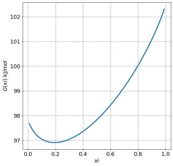
The minimum in the above plot is where \(\frac{\partial G}{\partial \xi}=0\) and indicates that the reaction is at equilibrium. We can determine this by perorming the differentiation, setting the derivative to 0, and solving for \(\xi\).

(4.476)\[\begin{eqnarray} \left( \frac{\partial G(\xi)}{\partial \xi}\right)_{T,P} &=& -\Delta G^\circ_{f,N_2O_4} + 2\Delta G^\circ_{f,NO_2} + -RT\ln\frac{1-\xi}{1+\xi} + (1-\xi)RT\frac{1+\xi}{1-\xi}\left( \frac{-1}{1+\xi} - \frac{1-\xi}{(1+\xi)^2}\right) + 2RT\ln \frac{2\xi}{1+\xi} + 2\xi RT \frac{1+\xi}{2\xi} \left( \frac{2}{1+\xi} - \frac{2\xi}{(1+\xi)^2}\right) \\ &=& -\Delta G^\circ_{f,N_2O_4} + 2\Delta G^\circ_{f,NO_2} + -RT\ln\frac{1-\xi}{1+\xi} + RT(1+\xi)\left( \frac{-1}{1+\xi} - \frac{1-\xi}{(1+\xi)^2}\right) + 2RT\ln \frac{2\xi}{1+\xi} + RT (1+\xi) \left( \frac{2}{1+\xi} - \frac{2\xi}{(1+\xi)^2}\right) \\ &=&-\Delta G^\circ_{f,N_2O_4} + 2\Delta G^\circ_{f,NO_2} - RT\ln\frac{1-\xi}{1+\xi} + 2RT\ln \frac{2\xi}{1+\xi} + RT\left( -1 - \frac{1-\xi}{1+\xi}\right) + RT \left( 2 - \frac{2\xi}{1+\xi}\right) \\ &=&-\Delta G^\circ_{f,N_2O_4} + 2\Delta G^\circ_{f,NO_2} - RT\ln\frac{1-\xi}{1+\xi} + 2RT\ln \frac{2\xi}{1+\xi} + RT\left( \frac{-(1+\xi) - (1-\xi)}{1+\xi}\right) + RT \left( \frac{2+2\xi - 2\xi}{1+\xi}\right) \\ &=&-\Delta G^\circ_{f,N_2O_4} + 2\Delta G^\circ_{f,NO_2} - RT\ln\frac{1-\xi}{1+\xi} + 2RT\ln \frac{2\xi}{1+\xi} + RT\left( \frac{-2}{1+\xi}\right) + RT \left( \frac{2}{1+\xi}\right) \\ &=&-\Delta G^\circ_{f,N_2O_4} + 2\Delta G^\circ_{f,NO_2} - RT\ln\frac{1-\xi}{1+\xi}+ 2RT\ln \frac{2\xi}{1+\xi} \\ &=& -\Delta G^\circ_{f,N_2O_4} + 2\Delta G^\circ_{f,NO_2} + RT\ln\left[ \left( \frac{2\xi}{1+\xi}\right)^2 \frac{1+\xi}{1-\xi}\right] \\ &=& -\Delta G^\circ_{f,N_2O_4} + 2\Delta G^\circ_{f,NO_2} + RT\ln\left[ \frac{4\xi^2}{(1+\xi)(1-\xi)}\right] \\ &=& -\Delta G^\circ_{f,N_2O_4} + 2\Delta G^\circ_{f,NO_2} + RT\ln\left[ \frac{4\xi^2}{1-\xi^2}\right] \end{eqnarray}\]

Setting this to zero and solving for \(\xi\) yields

(4.477)\[\begin{eqnarray} \left( \frac{\partial G(\xi)}{\partial \xi}\right)_{T,P}|_{eq} &=& 0 \\ &=& -\Delta G^\circ_{f,N_2O_4} + 2\Delta G^\circ_{f,NO_2} + RT\ln\left[ \frac{4\xi^2}{1-\xi^2}\right] \\ \Rightarrow \ln\left[ \frac{4\xi^2}{1-\xi^2}\right] &=& \frac{\Delta G^\circ_{f,N_2O_4} -2\Delta G^\circ_{f,NO_2} }{RT} \\ &=& -\frac{(2\Delta G^\circ_{f,NO_2} - \Delta G^\circ_{f,N_2O_4})}{RT} \\ &=& -\frac{\Delta G_{rxn}^\circ}{RT} \\ \Rightarrow \frac{4\xi^2}{1-\xi^2} &=& e^{-\frac{\Delta G_{rxn}^\circ}{RT}} = 0.1484 \end{eqnarray}\]

Solving this for \(xi\) yields

(4.478)\[\begin{equation} \xi_{eq} = 0.1891 \end{equation}\]

from scipy.optimize import fsolve
f = lambda x: np.exp(-(2*51.258-97.787)/(8.314/1000*298.15))*(1-x**2) - 4*x**2
fsolve(f,[0.1,0.4])

array([0.18914442, 0.18914442])

4.3.20.6. Equilibrium Constant and Temperature

The equilibrium constant depends on temperature. How it depends on temperature is given by the Van’T Hoff equation which can be derived from the Gibbs-Helmholtz equation.

(4.479)\[\begin{eqnarray} \left( \frac{\partial \Delta G^\circ/T}{\partial T}\right)_P &=& -\frac{\Delta H^\circ}{T^2} \\ \Rightarrow \left( \frac{\partial -RT\ln K_{eq}/T}{\partial T}\right)_P &=& -\frac{\Delta H^\circ}{T^2} \\ \Rightarrow \left( \frac{\partial \ln K_{eq}}{\partial T}\right)_P &=& \frac{\Delta H^\circ}{RT^2} \end{eqnarray}\]

We will now multiply by \(dT\) and integrate to investigate the behavior of \(K_{eq}\) with \(T\):

(4.480)\[\begin{eqnarray} d\ln K_{eq} &=& \frac{\Delta H^\circ}{RT^2} dT \quad \text{constant P} \\ \int d\ln K_{eq} &=& \frac{\Delta H^\circ}{RT^2} dT \quad \text{constant P} \\ \ln \frac{K_{eq}(T_2)}{K_{eq}(T_1)} &=& \int_{T_1}^{T_2} \frac{\Delta H^\circ}{RT^2} dT \quad \text{constant P} \end{eqnarray}\]

The above equation is the most general and allows for a temperature dependent \(\Delta H\). If, however, we assume it to be temperature indepedent we get

(4.481)\[\begin{equation} \ln \frac{K_{eq}(T_2)}{K_{eq}(T_1)} = -\frac{\Delta H^\circ}{R}\left(\frac{1}{T_2}-\frac{1}{T_1}\right) \end{equation}\]

This equation is the Van’t Hoff equation which demonstrates that an equation of \(\ln K\) vs \(\frac{1}{T}\) will be linear for \(\Delta H\) independent of temperature.

4.3.20.6.1. Example: Van’t Hoff

Given that \(\Delta H^\circ\) has an average value of \(-69.8\) kJ/mol over the temperature range \(500\) K to \(700\) K for the reaction

(4.482)\[\begin{equation} PCl_3(g) + Cl_2(g) \rightleftharpoons PCl_5(g) \end{equation}\]

estimate \(K_P\) at 700 K given that \(K_P = 0.0408\) at 500 K.

We will use the integrated Van’t Hoff equation above and solve for \(K(T_2)\):

(4.483)\[\begin{equation} K_P(T_2) = K_P(T_1)e^{-\frac{\Delta H^\circ}{R}\left(\frac{1}{T_2}-\frac{1}{T_1}\right)} \end{equation}\]

Now just plug in numbers and solve

(4.484)\[\begin{eqnarray} K_P(T_2) &=& (0.0408)e^{\frac{69.8\times10^3}{8.314}\left(\frac{1}{700}-\frac{1}{500}\right)} \\ &=& 3.34\times10^{-4} \end{eqnarray}\]

print(0.0408*np.exp(69.8e3/8.314*(1/700-1/500)))

0.00033664253542371996