import numpy as np
import matplotlib.pyplot as plt
%matplotlib inline
import plotting as myplt
---------------------------------------------------------------------------
ModuleNotFoundError                       Traceback (most recent call last)
Cell In[1], line 1
----> 1 import numpy as np
      2 import matplotlib.pyplot as plt
      3 get_ipython().run_line_magic('matplotlib', 'inline')

ModuleNotFoundError: No module named 'numpy'
4.3.9. Heat Engine Diagrams#
4.3.9.1. Learning goals#
After this class, students should be able to:
Draw a heat engine diagram for a heat engine and a refrigerator
Label \(w\), \(q_c\), \(q_h\), \(T_h\) and \(T_c\) on a heat engine diagram
Relate the above values to a \(PV\) digram for the same heat engine or refrigerator
Compute efficiency of heat engine
Compute coefficient of performance for a refrigerator
A heat engine diagram is another way of representing a heat engine. But before we get into these diagrams, some definitions:
A heat engine is a system that uses heat to generate work. A combustion engine is a prime example of a heat engine. In effect, heat transfers from a hot place to a cold place (spontaneous) and work is extracted along the way.
A refrigerator is something that uses work to move heat from a hot place to a cold place. Work is input to counteract the spontaneous flow of heat from the hot resevoir to the cold resevoir.
Heat engine diagrams are just another way to view the types of Thermodynamic cycles we have been talking about. The are used to indicate the flow of heat and work throughout the cycle.
To draw one, we start with three main components:
A motor (we draw as a circle)
A hot resevoir at \(T_2\) or \(T_h\)
A cold resevoir at \(T_1\) or \(T_c\)
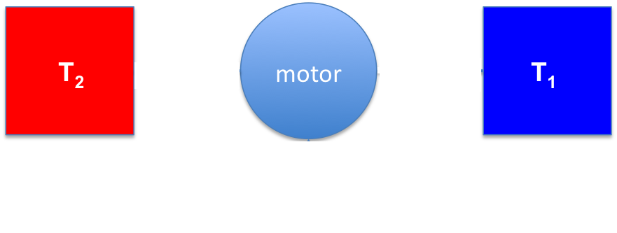
Arrows are then drawn to indicate the flow of heat and work. The direction of the arrows are what dictate whether we are looking at a heat engine or a refrigerator.
4.3.9.2. Heat Engine#
In a heat engine heat flow from a hot place to a cold place and work is extracted. On a heat engine diagram, this is indicated by three arrows:
\(q_2\) or \(q_h\) is the heat transferred from the hot resevoir to the motor
\(q_1\) or \(q_c\) is the heat transferred from the motor to the cold resevoir
\(w\) is the work extracted from the motor (motor is system so \(w<0\))
4.3.9.3. Refrigerator#
In a refrigerator work is input to move heat from a cold place to a hot place. On a heat engine diagram, this is indicated by three arrows:
\(w\) is done on the motor (motor is system so \(w>0\))
\(q_1\) or \(q_c\) is the heat extracted from the cold resevoir
\(q_2\) or \(q_h\) is the heat dumped into the hot resevoir
4.3.9.4. Relating Heat Engine Diagrams to \(PV\) diagrams#
In order to relate these two things, we must determine what \(q_c\) and \(q_h\) are on a \(PV\) diagram. This is most readily done for a Carnot cycle since \(q=0\) for the two adiabats. Thus, the only finite \(q\) values are from the two isotherms
4.3.9.5. Efficiencies of Heat Engines and COP of Refrigerators#
For a heat engine (\(w_{total}<0\)), the efficiency is the amount of work extracted, \(w_{total}\), divided by the energy in put, \(q_{in}\).
\(\varepsilon = \frac{w_{total}}{q_{in}}\)
For the Carnot cycle, this becomes:
\(\varepsilon = \frac{T_h-T_c}{T_h}\)
For a refrigerator (\(w_{total}>0\)), the coefficient of performance (COP) is the heat transferred from a cold place, \(q_c\), divided by the work done on the system.
\(COP = \frac{q_c}{w_{total}}\)
This value is maximized for a Carnot refrigerator so we know that:
\(COP \leq \frac{T_c}{T_h-T_c}\)
4.3.10. Entropy, a Molecular Persepective#
4.3.10.1. Learning goals#
After this class, students should be able to:
Describe what how entropy can drive certain outcomes
Compute entropy of a simple lattice gas
So far, we can summarize what we know about entropy as
Entropy is a state function.
Change in entropy is related to reversible heat and temperature.
Entropy is somehow related to disorder.
It is this last point that I want to focus on here.
4.3.10.2. Example: Galton Board#
To see how entropy, or disorder, plays a role in determining outcome let us consider the example of a galton board. In a Galton Board, balls are dropped from the top, through a peg board, finally landing in different bins on the bottom. This is likely familiar to you as a gameshow style game.
In the case of a Galton board, it is the gravitational potential energy difference between the top and the bottom that causes the balls to fall. There is no difference in potential energy, however, between any of the bins at the bottom. So why are certain bins (middle ones) favored?
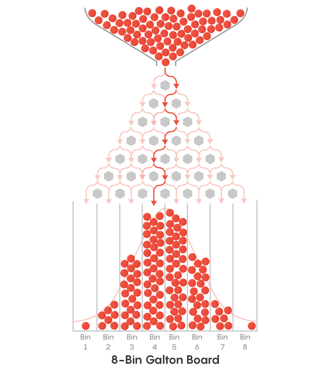
The reason is because the are more paths for the balls to get to the central bins than to the bins on the edge. You might recognize this as a bionomial process or the Fibonacci triangle. Regardless, the probability of the bins follow the binomial distribution.
If we consider a Galton board with just one peg and two bins, the probability of each bin is simple \(0.5\). More generally, the probability can be computed as:
\(P_{bin} = \frac{\text{Number of paths to that bin}}{\text{Total number of paths}}\)
In the case of a single peg, the are a total of two paths (left and right) and one path goes to the left (thus \(P_{left} = \frac{1}{2}\) and one path goes to the right.
If we go to the next level, there are two additional pegs followed by three bins at the bottom. The probability of each bin is:
Now, more generally, since these follow the binomal distribution, we can compute the probability of bin \(i\) given that there are \(n\) rows in the
where \(nCi\) is said as “\(n\) choose \(i\)” and \(nCi = \frac{n!}{(n-i)!i!}\).
4.3.10.3. Entropy and Counting#
So how does this relate to entropy? Entropy is not just the number of ways to get a certain outcome nor is it the probability of a certain outcome. It is, however, related to these quantities via the Boltzmann equation:
\(S = k\ln\Omega\)
where \(k\) is the Boltzmann constant and \(\Omega\) is the number of ways of arranging the system.
As a note, it is somtimes written \(S=k\ln W\) where \(W\) is substituted for \(\Omega\). There is no substantive difference between these equations.
4.3.10.4. Lattice Gas#
A lattice gas is a common example to see how the ideas of counting can be used to compute/estimate entropy for a molecular system. We will uses these examples to estimate entropy of mixing, for example. But we start by simply describing the lattice gas model.
Estimate the entropy of two molecules of an excluded volume gas in a fixed volume.
We currently have no tools that allow us to estimate the absolute entropy of a system (we might be able to compute change in entropy during a process)…
To estimate this, we consider the two molecules fixed in a 2D box (square):
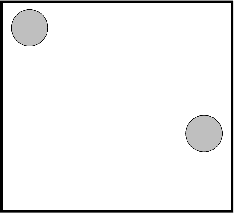
The gas particles can move around but cannot overlap (finite volume). So how many ways can we arrange them? Currently, their motion is on a continuous space and not possible to count. Instead, we discretize the space in some manner and say that the gas particles can occupy a single grid (or lattice) position
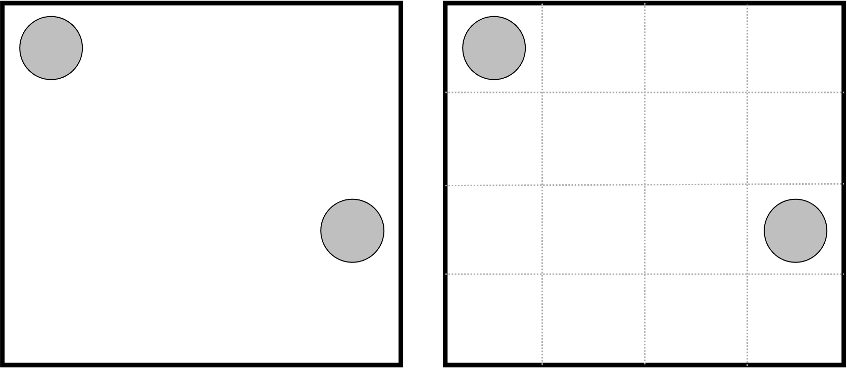
Now, the number of ways of arranging the gas particles (\(W\) or \(\Omega\) in the Boltzmann equation) can be computed using the binomial coefficient
import scipy.special
scipy.special.binom(16,2)
120.0
k = 1.38e-23 # this is in units of J/K
print(k*np.log(scipy.special.binom(16,2)))
---------------------------------------------------------------------------
NameError                                 Traceback (most recent call last)
<ipython-input-2-d79cf8b0e83e> in <module>
      1 k = 1.38e-23 # this is in units of J/K
----> 2 print(k*np.log(scipy.special.binom(16,2)))

NameError: name 'np' is not defined
4.3.10.4.1. A Note on Units of \(k\) (Boltzmann constant)#
\(k = 1.38\times10^{-23}\) \(J/K\) is a typical value and units of \(k\). Note that this is an extremely small value and that it is on the order of magnitude of a single particle/molecule. i.e. \(10^{-23}\) when Avogadro’s number is \(10^{23}\).
\(k\) can be thought of as the molecular value of the gas constant. So, if you want to compute a molar quantity, i.e. \(J/(K\cdot mol)\), you would use \(R = 8.314\) \(J/(K\cdot mol)\) for \(k\).
4.3.10.4.2. Entropy of Mixing of Two (or more) Lattice Gasses#
Given that we can now estimate the entropy of a lattice gas in a given volume, we can compute the change in entropy upon expansion, contraction or mixing of lattice gasses.
4.3.10.4.3. Example#
Consider the system of two distinguishable excluded volume gasses initially separated by a barrier indicated by the dashed line. Compute the change in entropy for the following system if the dashed line is made to be:
Permeable only to solid colored particles (semi-permeable)
Fully permeable
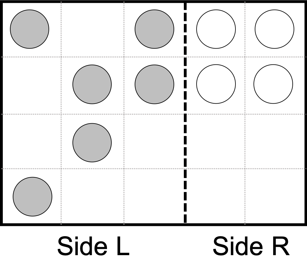
Permeable only to solid particles from Side L.
We start writing the entropy of mixing as:
So we need to compute \(W_f\) and \(W_i\). We start with \(W_i\):
print(scipy.special.binom(12,6))
print(scipy.special.binom(8,4))
print(scipy.special.binom(12,6)*scipy.special.binom(8,4))
924.0
70.0
64680.0
Now for \(W_f\). There are many ways to correctly think about and compute the number of ways to arrange this system. Here, I will consider the following decomposition
\(W_{open}\) is the number of ways to arrange the open circles. Since the open circles cannot diffuse across the barrier, this is identical to the initial situation. Thus,
\(W_{solid}\) is only slighty more complicated. Since the barrier is permeable to the solid particles, they can diffuse across it. Thus, nominally, the solid circles can be in any one of the 20 lattice positions. But, we know that the open circles are occupying four of these lattice positions, so really the solid circles have 16 lattice positions to choose from. Thus,
and
print(scipy.special.binom(16,6))
print(scipy.special.binom(16,6)*scipy.special.binom(8,4))
8008.0
560560.0
Finally, we compute \(\Delta S_{mix}\):
print(560560/64680)
print(np.log(560560/64680))
print(8.314*np.log(560560/64680))
8.666666666666666
2.159484249353372
17.953952049123934