4.4.3. Reversible Reactions

4.4.3.1. Motivation

Reactions that can proceed both in the forward and reverse directions are important in chemistry, as we saw in the equilibrium section of Thermodynamics. In these notes we will discuss how to write rate laws for simple “reversible” reactions.

4.4.3.2. Learning Goals

After working through these notes, you should be able to:

1. Define a reversible reaction in the context of kinetics

2. Write out the derivative of concentration with respect to time for species in reversible reactions

3. Derive and use the first order integrated rate law for a simple reversible process

4.4.3.3. Coding Concepts

The following coding concepts are used in this notebook:

1. Variables

2. Functions

3. Plotting with matplotlib

4.4.3.4. Rate Laws for Reversible Reactions

Most chemical processes should be considered to go both in the forward and reverse directions. In the context of Kinetics, we describe this as a reversible reaction (distinct from a reversible process in Thermodynamics). A reaction that is considered to go both in the forward and reverse direction is denoted with two arrows (as we have seen in the Equilibrium portion of the Thermodynamics section). As an example

(4.526)\[\begin{equation} A \overset{k_1}{\underset{k_{-1}}{\rightleftharpoons}} B \end{equation}\]

we say the \(A\) transforms to \(B\) with rate constant \(k_1\) and \(B\) transforms to \(A\) with rate constant \(k_{-1}\). In situations such as these we also can write the equilibrium constant, \(K_C\), as

(4.527)\[\begin{equation} K_C = \frac{[B]_{eq}}{[A]_{eq}} \end{equation}\]

To achieve equilibrium, we must allow the reaction to achieve the steady-state. That is, the concentrations of \([A]\) and \([B]\) must remain constant. This is noted mathematically as

(4.528)\[\begin{equation} \frac{d[A]}{dt} = \frac{d[B]}{dt} = 0 \end{equation}\]

Note that this does not mean that the forward and reverse reactions are not happening. It just means that they are happening in such a way that and \(A\) depleted in the forward process is created in equal amount by the reverse process. Thus, there is no net change in \([A]\) but the equilibrium is still dynamic.

We now consider the special case in which the forward and reverse processes are both first order. In such a case we can write

(4.529)\[\begin{eqnarray} v_{forward} = k_1[A] v_{backward} = k_{-1}[B] \end{eqnarray}\]

If we want to equate these rate laws to the time derivatives of concentration of \(A\), for example, we must take into account the forward and reverse processes simultaneously. That is, \(A\) will be depleted by the forward process but will also be created by the reverse process thus

(4.530)\[\begin{equation} \frac{d[A]}{dt} = -k_1[A] + k_{-1}[B] \end{equation}\]

Notice that the forward depletion is denoted by a negative sign infront of \(k_1[A]\) and the reverse creation is denoted by a positive sign infront of \(k_{-1}[B]\).

Notice that, at equilibrium, we have that \(\frac{d[A]}{dt}=0\) which yields

(4.531)\[\begin{eqnarray} \frac{d[A]}{dt} = 0 &=& -k_1[A]_{eq} + k_{-1}[B]_{eq} \\ \Rightarrow k_1[A]_{eq} = k_{-1}[B]_{eq} \\ \Rightarrow \frac{k_1}{k_{-1}} = \frac{[B]_{eq}}{[A]_{eq}} = K_C \end{eqnarray}\]

This is clearly an important relationship that states that the equilibrium constant is equal to a ratio of the forward and reverse rate constants. We will use this in our derivation below for the integrated rate law.

In order to derive an integrated rate law from the differential expression, we must write \([B]\) in terms of \([A]\). To achieve this, we regonize that the stoichiometry of the problem indicates that the total concentration of \([A] + [B]\) will remain constant and set by the initial concentrations of the experiment. Assume \([A] = [A]_0\) and \([B]=0\) at \(t=0\) thus \([B] = [A]_0-[A]\). Substituting this into the equation above yields

(4.532)\[\begin{eqnarray} \frac{d[A]}{dt} &=& -k_1[A] + k_{-1}([A]_0-[A]) \\ &=& -(k_1 + k_{-1})[A] + k_{-1}[A]_0 \\ \Rightarrow \frac{d[A]}{-(k_1 + k_{-1})[A] + k_{-1}[A]_0} &=& dt \\ \Rightarrow \int_{[A]_0}^{[A]_t} \frac{d[A]}{(k_1 + k_{-1})[A] - k_{-1}[A]_0} &=& -\int_0^tdt \\ \frac{1}{(k_1 + k_{-1})}\int_{k_1[A]_0}^{(k_1 + k_{-1})[A] - k_{-1}[A]_0} \frac{du}{u} &=& -t \end{eqnarray}\]

in the last step we have set \(u = (k_1 + k_{-1})[A] - k_{-1}[A]_0\) and thus \(du = (k_1 + k_{-1})d[A]\) or \(d[A] = \frac{du}{(k_1 + k_{-1})}\). The integral can be solved and simplified to

(4.533)\[\begin{eqnarray} \int_{k_1[A]_0}^{(k_1 + k_{-1})[A] - k_{-1}[A]_0} d\ln u &=& -(k_1 + k_{-1})t \\ \ln\left((k_1 + k_{-1})[A] - k_{-1}[A]_0\right) - \ln{k_1[A]_0} &=& -(k_1 + k_{-1})t \\ \ln\frac{(k_1 + k_{-1})[A] - k_{-1}[A]_0}{k_1[A]_0} &=& -(k_1 + k_{-1})t \\ \Rightarrow \frac{(k_1 + k_{-1})[A] - k_{-1}[A]_0}{k_1[A]_0} &=& e^{-(k_1 + k_{-1})t} \\ \frac{(k_1 + k_{-1})[A]}{k_1[A]_0} - \frac{k_{-1}[A]_0}{k_1[A]_0} &=& e^{-(k_1 + k_{-1})t} \\ \frac{[A]}{[A]_0} + \frac{1}{K_C}\frac{[A]}{[A]_0} - \frac{1}{K_C} &=& e^{-(k_1 + k_{-1})t} \\ \frac{[A]}{[A]_0} + \frac{[A]_{eq}}{([A]_0-[A]_{eq})}\frac{[A]}{[A]_0} - \frac{[A]_{eq}}{([A]_0-[A]_{eq})} &=& e^{-(k_1 + k_{-1})t} \\ \Rightarrow \frac{[A] ([A]_0-[A]_{eq}) + [A]_{eq}[A]}{([A]_0-[A]_{eq})[A]_0} &=& e^{-(k_1 + k_{-1})t} + \frac{[A]_{eq}}{([A]_0-[A]_{eq})} \\ \frac{[A]}{([A]_0-[A]_{eq})} &=& e^{-(k_1 + k_{-1})t} + \frac{[A]_{eq}}{([A]_0-[A]_{eq})} \\ \Rightarrow [A] &=& ([A]_0-[A]_{eq})e^{-(k_1 + k_{-1})t} + [A]_{eq} \end{eqnarray}\]

The final expression can be considered an integrated rate law for reversible first order processes. A slight rearrangement yields

(4.534)\[\begin{equation} \ln\left([A] - [A]_{eq}\right) = - (k_{1} + k_{-1})t + \ln\left([A]_0 - [A]_{eq}\right) \end{equation}\]

demonstrating that a plot of \(\ln\left([A] - [A]_{eq}\right) \) vs \(t\) should be linear with slope \(-(k_1 + k_{-1})\) and intercept \(\ln\left([A]_0 - [A]_{eq}\right)\).

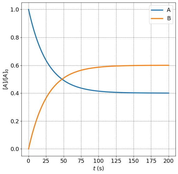
4.4.3.4.1. Example: Time Dependence of \([A]/[A]_0\) for Reversible First Order Processes

Consider a generic equilibrium

(4.535)\[\begin{equation} A \rightleftharpoons B \end{equation}\]

with \(k_1 = 2.25\times10^{-2}\) s\(^{-1}\) and \(k_2 = 1.50\times10^{-2}\) s\(^{-1}\). Plot the time depedence of the concentration of species \(A\) and species \(B\) starting with 100% of species \(A\).

We will need to do some slight rearrangements of the equation we have above to achieve this. First, we want to plot \([A]/[A]_0\) so we divide the equation above by \([A]_0\):

(4.536)\[\begin{eqnarray} \frac{[A]}{[A]_0} &=& \frac{([A]_0-[A]_{eq})e^{-(k_1 + k_{-1})t}}{[A]_0} + \frac{[A]_{eq}}{[A]_0} \\ \end{eqnarray}\]

Next, we recognize that by dictating the rate constants, the problem has also dictated the relative amounts of the species at equilibrium:

(4.537)\[\begin{eqnarray} \frac{B_{eq}}{A_{eq}} &=& K_C = \frac{k_1}{k_{-1}} \\ \frac{A_0 - A_{eq}}{A_{eq}} &=& K_C \\ A_0 &=& (K_C+1)A_{eq} \end{eqnarray}\]

Now we use this relationship in the equation for \([A]/[A]_0\) to get

(4.538)\[\begin{eqnarray} \frac{[A]}{[A]_0} &=& \frac{([A]_0-[A]_{eq})e^{-(k_1 + k_{-1})t}}{[A]_0} + \frac{1}{K_C+1} \\ \frac{[A]}{[A]_0} &=& \frac{K_C[A]_{eq}e^{-(k_1 + k_{-1})t}}{[A]_0} + \frac{1}{K_C+1} \\ \frac{[A]}{[A]_0} &=& \frac{K_Ce^{-(k_1 + k_{-1})t}}{K_C+1} + \frac{1}{K_C+1} \\ \end{eqnarray}\]

Now we can plot this function with just \(k_1\), \(k_{-1}\) and time as input.

Show code cell source Hide code cell source

import numpy as np
import matplotlib.pyplot as plt
%matplotlib inline
# setup plot parameters
fontsize=16
fig = plt.figure(figsize=(8,8), dpi= 80, facecolor='w', edgecolor='k')
ax = plt.subplot(111)
ax.grid(which='major', axis='both', color='#808080', linestyle='--')
ax.set_xlabel("$t$ (s)",size=fontsize)
ax.set_ylabel("$[A]/[A]_0$",size=fontsize)
plt.tick_params(axis='both',labelsize=fontsize)
def rev_first_order(t,k1,k2):  
    K = k1/k2
    return K*np.exp(-(k1+k2)*t)/(K+1) + 1/(K+1)
k1 = 2.25e-2
k2 = 1.50e-2
t = np.arange(0,200,0.01)
ax.plot(t,rev_first_order(t,k1,k2),lw=3, label="A")
ax.plot(t,1-rev_first_order(t,k1,k2),lw=3, label="B")
plt.legend(fontsize=16);