import numpy as np
import matplotlib.pyplot as plt
%matplotlib inline
import plotting as myplt
---------------------------------------------------------------------------
ModuleNotFoundError                       Traceback (most recent call last)
Cell In[1], line 1
----> 1 import numpy as np
      2 import matplotlib.pyplot as plt
      3 get_ipython().run_line_magic('matplotlib', 'inline')

ModuleNotFoundError: No module named 'numpy'
4.3.11. The Third Law of Thermodynamics#
Statement of the third law:
Entropy of a pure solid approaches zero as temperature approaches zero.
4.3.11.1. Learning goals#
After these notes, students should be able to:
Compute the entropy change for a heating or cooling a substance with constant heat capacity
Compute the entropy change for a heating or cooling a substance with temperature dependent heat capacity
Compute the heat required to raise or lower the temperature of a substance with constant heat capacity
Compute the heat required to raise or lower the temperature of a substance with temperature dependent heat capacity
Compute the heat and entropy of a substance undergoing a phase change.
This allows us to define absolute entropies. These are entropies of a substance as \(T\rightarrow 0\) K. Namely, we can define:
4.3.11.2. Entropies and Heat of Condensed Phase Systems#
So far we have been considering gas phase systems as examples in our section on Thermodynamics. But, as systems approach \(0\) K they are typically in the solid phase. So how to we compute entropies of these types of systems? A related question, how do we compute heat, \(q\), required to achieve a certain process for condensed phase systems?
4.3.11.2.1. Example: Heating a solid with a constant heat capacity#
Compute the heat, \(q\), and change in entropy, \(\Delta S\), to raise the temperature of a solid from \(10\) K to \(100\) K at constsant pressure given that \(\bar{C}_P = 50.0\) \(J\) \(K^{-1}\) \(mol^{-1}\).
Recall that \(\Delta H = q_p\), so we need to compute the change in enthalpy at constant pressure. We start by writing out the following differential form of enthalpy in terms of variables \(T\) and \(P\):
Since this is a constant pressure process, \(dP=0\). Thus, we now have:
Notice that the integrand, \(\left(\frac{\partial H}{\partial T}\right)_P=C_P\), is the heat capacity at constant pressure.
We now plug in our values from the problem:
50*(100-10)
4500
Now for change in entropy. Again, we start with the differential form and then we are going to integrate:
where the last equality holds for heat at constant pressure. Now we plug in \(dH = C_P dT\):
Since heat capacity in this problem is temperature independent, it can be pulled out of the integral.
50*np.log(100/10)
115.12925464970229
4.3.11.2.2. Example: Heating a solid with a temperature dependent heat capacity#
Compute the heat, \(q\), and change in entropy, \(\Delta S\), to raise the temperature of a solid from \(10\) K to \(100\) K at constsant pressure given that \(\bar{C}_P = 5.0\cdot T^2\) \(J\) \(K^{-1}\) \(mol^{-1}\).
Since the heat capacity is temperature dependent, we must take that into account when doing the integral to compute \(q\). Start with the integral form of \(q\):
5/3*(100**3-10**3)
1665000.0
Now \(\Delta S\):
5/2*(100**2-10**2)
24750.0
4.3.11.3. Entropies and Heat of Phase Changes#
The previous examples assumed that the system/material remained in the same phase during the heating process. We would like to, however, be able to compute how much heat is required to melt or vaporize a substance too. We would also like to know the change in entropy in doing so.
4.3.11.3.1. Example - Entropy and Heat of Phase Change#
Compute the heat required, \(q\), and change in entropy, \(\Delta S\), to take a substance from \(90\) K to \(110\) K under constant pressure conditions. The melting temperature of the substance is \(100\) K and the heat of fusion is \(\Delta H_{fusion} = 0.25 \) \(kJ/mol\). Additionally, the heat capacity of the solid is \(\bar{C}_{P,s} = 30\) \(J/(K\cdot mol)\) and the heat capacity of the liquid is \(\bar{C}_{P,l} = 15\) \(J/(K\cdot mol)\)
def plot_Cp_v_T(Ts,Cps,Tf,Tl,Cpl):
    fig, ax = myplt.define_figure(xlabel="T (K)",ylabel="C$_P$ (J/mol/K)")
    ax.plot(Ts,Cps*np.ones(Ts.size),lw=3,label="Solid")
    ax.plot(Tl,Cpl*np.ones(Tl.size),lw=3,label="Liquid")
    ax.set_ylim(0,31)
    plt.legend(fontsize=16)
plot_Cp_v_T(np.arange(90,100,0.1),30,100,np.arange(100,110,0.1),15)
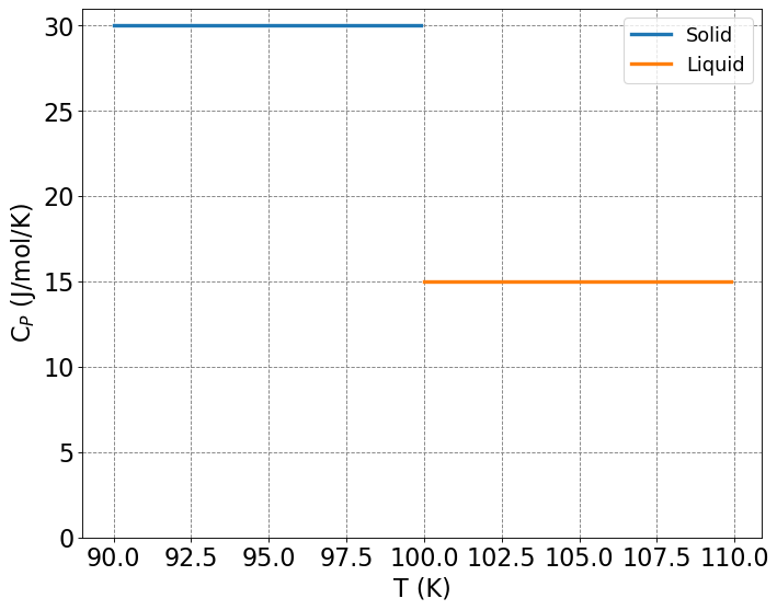
The above is a plot of \(C_P\) as a function of \(T\). We see that there is a discontinuity at \(T=100\) K, the melting temperature of this substance.
We start as we did before by writing down the integral form of \(q\) or \(\Delta H\)
Since the heat capacities change at the melting temperature, there is a discontinuity in the function \(C_p(T)\). In order to account for this in the above integral, we must split the integral into two parts.
Note that we have to add \(\Delta H_{fusion}\). You can essentially think of this as the integral evaluated at \(T=T_{melt}\). Now, since both heat capacities are constant w.r.t. \(T\), we get:
def plot_q_v_T(Ts,Cps,Tf,dHf,Tl,Cpl,Ti):
    fig, ax = myplt.define_figure(xlabel="T (K)",ylabel="q (J/mol)")
    ax.plot(Ts,Cps*(Ts-Ti),lw=3,label="Solid")
    ax.plot(Tf*np.ones(100),np.arange(Cps*(Tf-Ti),Cps*(Tf-Ti)+dHf,dHf/100.0),lw=3,label="Fusion (Melting)")
    ax.plot(Tl,Cpl*(Tl-Ti)+Cps*(Tf-Ti)+dHf-Cpl*(Tf-Ti),lw=3,label="Liquid")
    plt.legend(fontsize=16)
plot_q_v_T(np.arange(90,100,0.1),30,100,250,np.arange(100,110,0.1),15,90)
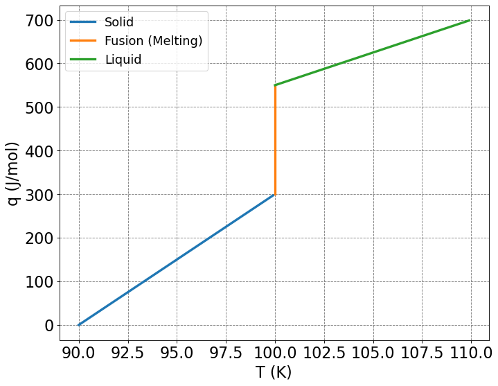
The above is a plot pf \(q(T)\). The amount of heat required to raise the temperature of the solid increases steadily from \(90\) K to \(100\) K and the slope is \(C_{P,s}=30\) \(J/mol/K\). The vertical increase in the amount of heat required to raise the temperature above \(100\) K is due to the melting of the substance at this temperature. Melting requires an input of heat distinct from the heat capacities. The amount of heat required to raise the temperature of the liquid increases steadily from \(100\) K to \(110\) K and the slope is \(C_{P,s}=15\) \(J/mol/K\).
Now, to wrap up \(q\) we simply plug in our numbers. Be careful about units!
30*(100-90) + 250 + 15*(110-100)
700
What about \(\Delta S\)? Again, we start with the integral form and split the integral over the discontuity:
30*np.log(100/90) + 250/100 + 15*np.log(110/100)
7.090468166799665