4.5.21. H\(_2\) Configuration Interaction#
4.5.21.1. Motivation:#
We saw in the notes on H\(_2\) in a minimal basis that single determinant methods, such as the one presented, do no accurately capture molecular dissociation. Here I will present the configuration interaction method in the same minimal basis as a way to capture the correct dissociation behavior.
4.5.21.2. Learning Goals:#
After working through these notes, you will be able to:
Describe how the Configuration Interaction method achieves the correct dissociation limit for H\(_2\)
Define the steps for performing a CI calculation for H\(_2\) in a minimal basis
Identify the bond distance and bond energy on a plot of E vs R for H\(_2\).
Identify the correct variational parameter for the CI calculation of H\(_2\) in a minimal basis as \(R\rightarrow\infty\)
4.5.21.3. Coding Concepts:#
The following coding concepts are used in this notebook:
4.5.21.4. Background#
Recall that the bonding orbital for H\(_2\) in a minimal 1s basis can be written as
The first two terms in the numerator of the last expression represent the correct dissociation limit (the separated neutral H atoms) while the last two terms in the numerator represent a hydride ion and a proton.
In order to get the correct dissociation limit with this type of wave function, we need a way of eliminating the contribution from \(1s_A(1)1s_A(2) + 1s_B(1)1s_B(2)\) as \(R\rightarrow\infty\). These contributions are important at small \(R\) so we cannot simply remove them from our trial wave function.
The Configuration Interaction method is a linear variational method in which we introduce additional molecular-orbital based wavefunctions beyond just the bonding orbital. To simplify things a bit, we need only consider the doubly populated bonding and doubly populated antibonding molecular orbitals in the minimal basis picture and thus we will consider a new trial wave function that is of the form:
where \(\sigma_a\) is the antibonding orbital and is given by
In order to see how this method allows us to eliminate the ionic portion of the \(\sigma_b\sigma_b\) wave function we need to expand both terms in the \(CI\) wave function.
As \(R\rightarrow\infty\) we have \(S\rightarrow0\) and thus the \(CI\) wavefunction becomes:
We now see that the wavefunction terms multiplied by \((c_1+c_2)\) are for electrons sitting on different nuclei while the terms multiplied by \((c_1-c_2)\) are for electrons sitting on the same nuclei (the ionic terms). Since \(c_1+c_2\) and \(c_1-c_2\) are linearly independent, these two coefficients are distinct that thus the ionic contribution can be eliminated if energetically desired.
4.5.21.5. The CI Method#
The CI method is based on the linear variational parameter method. That is, we will need to populate an \(H\) matrix and an \(S\) matrix and then diagonalize \(S^{-1}H\). In this case, however, the energy (smallest eigenvalue of the \(S^{-1}H\) matrix) will end up being a function that depends on \(Z\) which we will minimize with respect to \(Z\). Otherwise the procedure is identical to what we have done before.
We start by expressing the wave function again as
4.5.21.5.1. The \(S\) Matrix#
We start by populating the \(S\) matrix:
The \(\sigma_b\) orbitals are normalized as defined above thus this term is 1. Similarly
Now for the cross term
Thus, the \(S\) matrix is
and conveniently
4.5.21.5.2. The \(H\) Matrix#
The \(H\) matrix is a bit more involved than the \(S\) matrix.
We start by populating the matrix:
This is just the ground state energy of the H\(_2\) molecule in this minimal basis on was given in the previous notes (not derived) and provided here as well:
The \(H_{22}\) element is of a similar form but not exactly the same (It should be a higher energy since it isn’t the ground state and is an antibonding orbital):
The \(H_{12}\) element is
All of the integrals (\(S(R)\), \(J(R)\), \(K(R)\), \(J'(R)\), \(K'(R)\) and \(L(R)\)) are given in a table in the previous notes.
4.5.21.5.3. Diagonalizing the \(S^{-1}H\) Matrix#
Now that we have the two matrices populated, we can diagonlize the matrices. To make things slightly complicated, the \(H\) matrix elements are functions of both \(Z\) and \(R\) so we cannot simply determine the value of the energy unless we are given specific values for these. While this is certainly feasible for \(R\) (indeed the Born-Oppenheimer approximation is such that we need to solve the Schrodinger equation at a given value for \(R\)) we really want to minimize the energy with respect to \(Z\) so we need to determine the minimal eigenvalue of the matrix as a function of both \(R\) and \(Z\).
To do so, I will use generic expression for the matrix elements of the Hamiltonian and only plug in the formulas above in the code below when I actually solve for numbers.
We can now solve for the eigenvalues using the determinant of \(S^{-1}H-\lambda I\):
Solving for the roots of this quadratic equation yields
From this equation (and the equations for the \(H\) matrix elements and all of the integral equations) we can solve for the \(CI\) energy at a given \(R\) and \(Z\). Notice that we will get two energies, one from the \(+\) and one from the \(-\). In this case, the thing being added or subtracted is always positive so the \(-\) is the lower energy.
Below I have code to compute this quantity as a function of \(R\) and \(Z\). I compute this for \(Z=1\) as well as minimize \(E\) w.r.t \(Z\) at each value of \(R\). In that case I use a numeric minimization procedure provided in the scipy python package.
Show code cell source
# configuration interaction for H2 in minimal basis
# H2 MO Minimal Basis
from scipy.optimize import minimize
from scipy import integrate
import matplotlib.pyplot as plt
%matplotlib inline
import numpy as np

gamma = 0.57721

def J(R):
    return np.exp(-2*R)*(1+1/R) - 1/R
def K(R):
    return -np.exp(-R)*(1+R)
def S(R):
    return np.exp(-R)*(1 + R + R*R/3)
def S2(R):
    return np.exp(R)*(1 - R + R*R/3)
def E1_integrand(t):
    return np.exp(-t)/t
def E1(x):
    return integrate.quad(E1_integrand,x,np.infty)[0]
def J2(R):
    return 1/R - np.exp(-2*R) * (1/R + 11/8 + 0.75*R + R*R/6)
def L(R):
    return np.exp(-R) * (R + 1/8 + 5/(16*R)) + np.exp(-3*R)*(-1/8 - 5/(16*R))
def K2(R):
    term_1 = -0.2 * np.exp(-2*R) * (-25/8 + 23*R/4 + 3*R*R + R**3/3)
    term_2 = 1.2/R * (S(R)**2 * (gamma + np.log(R)) - S2(R)**2 * E1(4*R) + 2*S(R) * S2(R) * E1(2*R))
    return term_1+term_2

def H11(Z,R):
    w = Z*R
    denom = 1+S(w)
    prefactor = Z/denom
    term1 = Z*(1 - S(w) - 2*K(w))
    term2 = -2 + 2*J(w) + 4*K(w)
    term3 = (5/16 + 0.5*J2(w) + K2(w) + 2*L(w))/denom
    return prefactor*(term1 + term2 + term3) + 1/R

def H22(Z,R):
    w = Z*R
    denom = 1-S(w)
    prefactor = Z/denom
    term1 = Z*(1 + S(w) + 2*K(w))
    term2 = -2 + 2*J(w) - 4*K(w)
    term3 = (5/16 + 0.5*J2(w) + K2(w) - 2*L(w))/denom
    return prefactor*(term1 + term2 + term3) + 1/R

def H12(Z,R):
    w = Z*R
    return Z*(5/16-0.5*J2(w))/(1-(S(w)**2))

def E_CI(Z,R):
    w = Z*R
    term1 = H11(Z,R) + H22(Z,R)
    term2 = np.sqrt((H11(Z,R) - H22(Z,R))**2 + 4*H12(Z,R)**2)
    return 0.5*(term1 - term2)

def E(Z,R):
    w = Z*R
    denom = 1+S(w)
    prefactor = Z/denom
    t1 = Z*(1-S(w)-2*K(w))
    t2 = -2 + 2*J(w) + 4*K(w)
    t3 = (5/16 + 0.5*J2(w) + K2(w) + 2*L(w))/denom
    return prefactor*(t1+t2+t3) + 1/R

# compute energy as function of R
R = np.arange(0.5,8,0.01)
E_1s_basis = np.empty(R.size)
E_1s_opt = np.empty(R.size)
E_CI_Z_1 = np.empty(R.size)
E_CI_Z_opt = np.empty(R.size)
Z_min_CI = np.empty(R.size)
Z_min_MO = np.empty(R.size)
for i, r in enumerate(R):
    E_1s_basis[i] = E(1,r)
    Z_min_MO[i] = minimize(E,1.0,args=(r)).x[0]
    E_1s_opt[i] = E(Z_min_MO[i],r)
    E_CI_Z_1[i] = E_CI(1,r)
    Z_min_CI[i] = minimize(E_CI,1.0,args=(r)).x[0]
    E_CI_Z_opt[i] = E_CI(Z_min_CI[i],r)
---------------------------------------------------------------------------
ModuleNotFoundError                       Traceback (most recent call last)
Cell In[1], line 3
      1 # configuration interaction for H2 in minimal basis
      2 # H2 MO Minimal Basis
----> 3 from scipy.optimize import minimize
      4 from scipy import integrate
      5 import matplotlib.pyplot as plt

ModuleNotFoundError: No module named 'scipy'
# configuration interaction for H2 in minimal basis
# H2 MO Minimal Basis
from scipy.optimize import minimize
from scipy import integrate
import matplotlib.pyplot as plt
%matplotlib inline
import numpy as np

gamma = 0.57721

def J(R):
    return np.exp(-2*R)*(1+1/R) - 1/R
def K(R):
    return -np.exp(-R)*(1+R)
def S(R):
    return np.exp(-R)*(1 + R + R*R/3)
def S2(R):
    return np.exp(R)*(1 - R + R*R/3)
def E1_integrand(t):
    return np.exp(-t)/t
def E1(x):
    return integrate.quad(E1_integrand,x,np.infty)[0]
def J2(R):
    return 1/R - np.exp(-2*R) * (1/R + 11/8 + 0.75*R + R*R/6)
def L(R):
    return np.exp(-R) * (R + 1/8 + 5/(16*R)) + np.exp(-3*R)*(-1/8 - 5/(16*R))
def K2(R):
    term_1 = -0.2 * np.exp(-2*R) * (-25/8 + 23*R/4 + 3*R*R + R**3/3)
    term_2 = 1.2/R * (S(R)**2 * (gamma + np.log(R)) - S2(R)**2 * E1(4*R) + 2*S(R) * S2(R) * E1(2*R))
    return term_1+term_2

def H11(Z,R):
    w = Z*R
    denom = 1+S(w)
    prefactor = Z/denom
    term1 = Z*(1 - S(w) - 2*K(w))
    term2 = -2 + 2*J(w) + 4*K(w)
    term3 = (5/16 + 0.5*J2(w) + K2(w) + 2*L(w))/denom
    return prefactor*(term1 + term2 + term3) + 1/R

def H22(Z,R):
    w = Z*R
    denom = 1-S(w)
    prefactor = Z/denom
    term1 = Z*(1 + S(w) + 2*K(w))
    term2 = -2 + 2*J(w) - 4*K(w)
    term3 = (5/16 + 0.5*J2(w) + K2(w) - 2*L(w))/denom
    return prefactor*(term1 + term2 + term3) + 1/R

def H12(Z,R):
    w = Z*R
    return Z*(5/16-0.5*J2(w))/(1-(S(w)**2))

def E_CI(Z,R):
    h11 = H11(Z,R)
    if not np.isscalar(h11): h11 = h11[0]
    h12 = H12(Z,R)
    if not np.isscalar(h12): h12 = h12[0]
    h22 = H22(Z,R)
    if not np.isscalar(h22): h22 = h22[0]
    Hmat = np.array([[h11, h12],[h12, h22]])
    e, v = np.linalg.eigh(Hmat)
    return e[0]

def E(Z,R):
    w = Z*R
    denom = 1+S(w)
    prefactor = Z/denom
    t1 = Z*(1-S(w)-2*K(w))
    t2 = -2 + 2*J(w) + 4*K(w)
    t3 = (5/16 + 0.5*J2(w) + K2(w) + 2*L(w))/denom
    return prefactor*(t1+t2+t3) + 1/R

# compute energy as function of R
R = np.arange(0.5,8,0.01)
E_1s_basis = np.empty(R.size)
E_1s_opt = np.empty(R.size)
E_CI_Z_1 = np.empty(R.size)
E_CI_Z_opt = np.empty(R.size)
Z_min_CI = np.empty(R.size)
Z_min_MO = np.empty(R.size)
for i, r in enumerate(R):
    E_1s_basis[i] = E(1,r)
    Z_min_MO[i] = minimize(E,1.0,args=(r)).x[0]
    E_1s_opt[i] = E(Z_min_MO[i],r)
    E_CI_Z_1[i] = E_CI(1,r)
    Z_min_CI[i] = minimize(E_CI,1.0,args=(r)).x[0]
    E_CI_Z_opt[i] = E_CI(Z_min_CI[i],r)
Show code cell source
fig, ax = plt.subplots(figsize=(8,6),dpi= 80, facecolor='w', edgecolor='k')
plt.tick_params(axis='both',labelsize=20)
plt.grid( which='major', axis='both', color='#808080', linestyle='--')
ax.plot(R,E_CI_Z_1,lw=4, label=r'$E_{CI}$ - $Z = 1$')
ax.plot(R,E_CI_Z_opt,lw=4, label=r'$E_{CI}$ - $Z = opt$')
ax.plot(R,E_1s_basis,lw=4, label=r'$E_{MO}$ - $Z=1$')
ax.plot(R,E_1s_opt,lw=4, label=r'$E_{MO}$ - $Z= opt$')
ax.set_xlabel(r'R/$a_0$',fontsize=20)
ax.set_ylabel(r'$E_0 (Hartree)$',fontsize=20)
plt.legend(fontsize=20)
ax2 = ax.twinx()
color = 'tab:orange'
ax2.set_ylabel('Z/e', color='gray', fontsize=20)  # we already handled the x-label with ax1
ax2.plot(R, Z_min_CI, '--', lw=3, color=color, alpha=0.75)
ax2.plot(R, Z_min_MO, '--', lw=3, color='tab:red', alpha=0.75)
ax2.tick_params(axis='y', labelcolor='gray',labelsize=20)
fig.tight_layout()
plt.title(r'Configuration Interaction Solution to the H$_2$ Molecule in Minimal Slater Basis',fontsize=16)
plt.show();
Show code cell source
min_index = np.argmin(E_CI_Z_1)
print("Bonding energy (Z=1):", np.round(E_CI_Z_1[min_index],5), "Hartree")
print("Bonding distance (Z=1):", np.round(R[min_index],5), "Bohr")
min_index = np.argmin(E_CI_Z_opt)
print("Bonding energy (Z=opt):", np.round(E_CI_Z_opt[min_index],5), "Hartree")
print("Bonding distance (Z=opt):", np.round(R[min_index],5), "Bohr")
print("Z at bond distance:", np.round(Z_min_CI[min_index],5), "e")
print("Difference from Exp: (kcal/mol):",np.round((E_CI_Z_opt[min_index]+1.174)*627.5895,2))
Bonding energy (Z=1): -1.11865 Hartree
Bonding distance (Z=1): 1.67 Bohr
Bonding energy (Z=opt): -1.14794 Hartree
Bonding distance (Z=opt): 1.43 Bohr
Z at bond distance: 1.19388 e
Difference from Exp: (kcal/mol): 16.36
4.5.21.5.4. The Results#
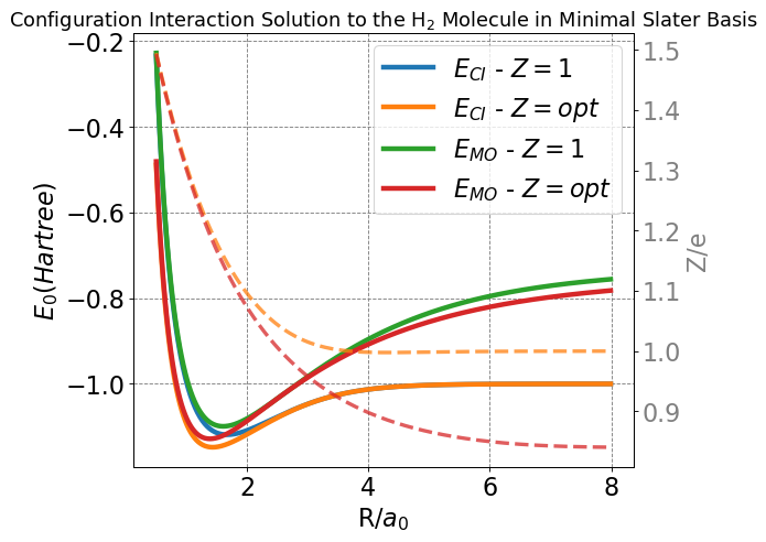
The blue (\(Z=1\)) and orange (\(Z=opt\)) curves in the plot above correspond to the CI solution in this minimal basis. Both curves go to the correct asymptotic limit of \(E=-1\) Hartree as \(R\rightarrow\infty\). This is as compared to the simple single MO picture the energy for which is plotted in the green curve (\(Z=1\)) which does not properly dissociate.
Additionally, I have plotted the optimal \(Z\) at each value of \(R\) for both the MO and CI pictures in dashed lines (and the corresponding charge is on the right-hand y-axis). We see that \(CI\) curve (orange) also goes to the correct asymptotic limit of \(Z=1\) as \(R\rightarrow\infty\). The MO curve (red) does not as we have previously discussed.
Finally, we can also look at the CI predicted energy at position of the minimum of the H\(_2\) molecule. These are
The energy is a modest improvement over the optimized MO calculation though the bond distance is now over estimated by 0.29 Bohr.
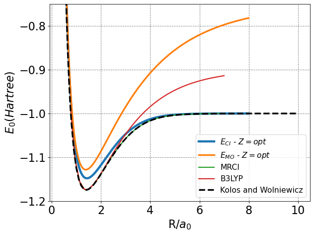
Below I also include a plot of \(E\) vs \(R\) of H\(_2\) for various methods including the optimized \(CI\) method, the optimized \(MO\) method, and the essentially exact Kolos and Wolniewicz data.
You can improve the CI estimate for the energy and bond distance by adding polarization functions to the basis and/or including additional terms in the basis. We will not do that, however. The MRCI method plotted below includes both of these.
fig, ax = plt.subplots(figsize=(8,6),dpi= 80, facecolor='w', edgecolor='k')
plt.tick_params(axis='both',labelsize=20)
plt.grid( which='major', axis='both', color='#808080', linestyle='--')
ax.plot(R,E_CI_Z_opt,lw=4, label=r'$E_{CI}$ - $Z = opt$')
ax.plot(R,E_1s_opt,lw=3, label=r'$E_{MO}$ - $Z= opt$')
ax.set_xlabel(r'R/$a_0$',fontsize=20)
ax.set_ylabel(r'$E_0 (Hartree)$',fontsize=20)
h2_all = np.loadtxt("h2_various_methods.txt",skiprows=1)
ax.plot(h2_all[:,0]*1.88973,h2_all[:,6],lw=2,label='MRCI')
ax.plot(h2_all[:,0]*1.88973,h2_all[:,7],lw=2,label='B3LYP')
exact = np.loadtxt("h2_kolos_wolniewicz.txt",skiprows=1)
ax.plot(exact[:,0],exact[:,1],'--',lw=3,c='k',label="Kolos and Wolniewicz")
ax.set_ylim(-1.2,-0.75)
ax.legend(fontsize=14)
plt.tight_layout()
plt.show();