4.5.27. Rigid Rotator

We have already looked at the vibrations of a diatomic molecule. Now we turn our attention to the rotations of a diatomic molecule. We will first consider the bond to be rigid (no vibration). We will investigate later how these two things can couple together. We consider the rotation of a diatomic molecule with two masses, \(m_1\) and \(m_2\), around the center-of-mass (C.O.M.) of the molecule.

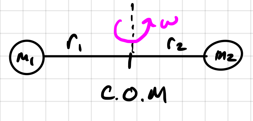
Given the above depiction of the system, we can define some important relationships.

\(\mu = \frac{m_1m_2}{m_1+m_2}\)

\(r_0 = r_1 + r_2\)

\(m_1r_1 = m_2r_2\)

\(KE = \frac{1}{2}m_1r_1\omega^2 + \frac{1}{2}m_2r_2\omega^2 = \frac{1}{2}(m_1r_1^2+m_2r_2^2)\omega^2 = \frac{1}{2}Iw^2\)

where \(I\) is the moment of intertia

\(I = m_1r_1^2+m_2r_2^2 = \mu r_0^2\)

Where the last two relationships lead to the conclusion that this problem can be reduced to a one-body like problem with \(KE = \frac{1}{2}\mu r_0^2 \omega^2\).

We now introduce the concept of angular momentum, \(\mathbf{L}= \mathbf{r} \times \mathbf{p}\). For rotation, it can be shown that \(\mathbf{L} = L = I\omega\). Thus the kinteic energy operator can be rewritten as

\(KE = \frac{L^2}{2I}\).

We must now consider the motion of the reduced mass on a sphere in a quantum mechanical way. We start by writing out the Hamiltonian

\(\hat{H} = \hat{K} + \hat{V} = -\frac{\hbar^2}{2\mu}\nabla_{xyz}^2+V(x,y,z)\).

where \(\nabla_{xyz}^2\) is the Laplacian operator in cartesian coordinates,

\( \nabla_{xyz}^2 = \frac{\partial^2}{\partial x} + \frac{\partial^2}{\partial y} + \frac{\partial^2}{\partial z}\).

Since we are considering only motion on a sphere it will be convenient to change to spherical polar coordinates.

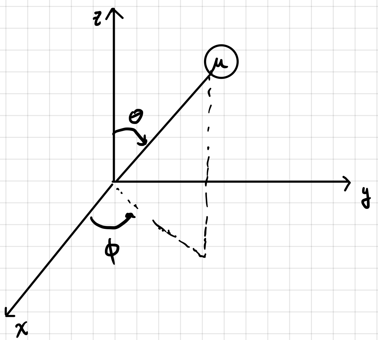
Converting the \(\nabla^2\) operator into spherical coordinates is a pain but it is

\(\nabla^2_{r\theta\phi} = \frac{1}{r^2}\frac{\partial}{\partial r}\left(r^2\frac{\partial}{\partial r}\right) + \frac{1}{r^2\sin\theta}\frac{\partial}{\partial\theta}\left(\sin\theta\frac{\partial}{\partial\theta}\right)+\frac{1}{r^2\sin^2\theta}\frac{\partial^2}{\partial^2\phi}\).

Also note that since we are restricting the bond vibration to be zero the potential in this problem is zero. Thus, in spherical coordinates with zero potential, we have a Schrodinger equation

\( -\frac{\hbar^2}{2\mu}\left[\frac{1}{r^2}\frac{\partial}{\partial r}\left(r^2\frac{\partial}{\partial r}\right) + \frac{1}{r^2\sin\theta}\frac{\partial}{\partial\theta}\left(\sin\theta\frac{\partial}{\partial\theta}\right)+\frac{1}{r^2\sin^2\theta}\frac{\partial^2}{\partial^2\phi}\right] \psi(r,\theta,\phi) = E \psi(r,\theta,\phi)\).

Note that since \(r\) does not change (bond doesn’t vibrate), we can write \(\psi(r_0,\theta,\phi) = BY(\theta,\phi)\) where \(B\) is a constant. We will thus try and solve for functions \(Y(\theta,\phi)\). Also, all \(\frac{\partial}{\partial r}\) terms go to zero. So now we have

\( -\frac{\hbar^2}{2\mu r_0^2}\left[\frac{1}{\sin\theta}\frac{\partial}{\partial\theta}\left(\sin\theta\frac{\partial}{\partial\theta}\right)+\frac{1}{\sin^2\theta}\frac{\partial^2}{\partial^2\phi}\right] Y(\theta,\phi) = E Y(\theta,\phi)\).

Note that \(\mu r_0^2 = I\). We will solve this problem by the method of separation of variables. The Schrodinger equation can be algebraically rearranged to give us

\( \left[\sin\theta\frac{\partial}{\partial\theta}\left(\sin\theta\frac{\partial}{\partial\theta}\right)+\frac{2IE}{\hbar^2}\sin^2\theta \right] Y(\theta,\phi) = -\frac{\partial^2}{\partial^2\phi} Y(\theta,\phi)\).

We now substitue \(Y(\theta,\phi) = \Theta(\theta)\Phi(\phi)\) and \(\beta = \frac{2IE}{\hbar^2}\) to get

\( \left[\sin\theta\frac{\partial}{\partial\theta}\left(\sin\theta\frac{\partial}{\partial\theta}\right)+\beta\sin^2\theta \right] \Theta(\theta)\Phi(\phi) = -\frac{\partial^2}{\partial^2\phi} \Theta(\theta)\Phi(\phi)\).

Divide both sides of the equation above by \(\Theta(\theta)\Phi(\phi)\) and note that the operator on the right-hand side is independent of \(\theta\) to yield

\( \frac{\sin\theta}{\Theta(\theta)}\frac{\partial}{\partial\theta}\left(\sin\theta\frac{\partial}{\partial\theta}\right)\Theta(\theta)+\beta\sin^2\theta = -\frac{1}{\Phi(\phi)}\frac{\partial^2}{\partial^2\phi} \Phi(\phi)\).

Now the left-hand side is independent of \(\phi\) and the right-hand side is independent of \(\theta\). Since these two things are equal but independent of the other’s variable they must be constant. We will define this constant as \(m^2\) (for reasons that will become clear later) and solve the following two equations independently

\(m^2 = -\frac{1}{\Phi(\phi)}\frac{\partial^2}{\partial^2\phi} \Phi(\phi) \tag{1}\)

\(m^2 = \frac{\sin\theta}{\Theta(\theta)}\frac{\partial}{\partial\theta}\left(\sin\theta\frac{\partial}{\partial\theta}\right)\Theta(\theta)+\beta\sin^2\theta \tag{2}\)

4.5.27.1. Solutions to \(\phi\) equation (1)

Equation (1) above can me simply rearranged to give

\(-m^2 \Phi(\phi)= \frac{\partial^2}{\partial^2\phi} \Phi(\phi)\)

which is straightforward eigenvalue-eigenvector problem with solutions

\(\Phi(\phi) = A_me^{im\phi}\quad \mathrm{and}\quad A_{-m}e^{-im\phi}\).

Applying boundary conditions, \(\Phi(\phi+2\pi) = \Phi(\phi)\) yields the quantization

\(m=0,\pm 1, \pm 2, ...\)

Thus we can write

\(\Phi(\phi) = Ae^{im\phi} \quad m=0,\pm 1, \pm 2, ...\).

Normalization yields \(A=\frac{1}{\sqrt{2\pi}}\).

4.5.27.2. Solutions to \(\theta\) equation (2)

The solutions to equation (2) above are not as straightforward as those for equation (1). We start by rewriting the original equation here:

\(m^2 = \frac{\sin\theta}{\Theta(\theta)}\frac{\partial}{\partial\theta}\left(\sin\theta\frac{\partial}{\partial\theta}\right)\Theta(\theta)+\beta\sin^2\theta\).

Now make a change of variable \(x = \cos\theta\) which yields \(\frac{dx}{-\sin\theta}=d\theta\) and define \(P(x) = \Theta(\theta)\). Plugging these in an performing some rearrangements yields the Legendre equation

\((1-x^2)\frac{d^2}{dx^2}P(x)-2x\frac{d}{dx}P(x)+\left[\beta-\frac{m^2}{1-x^2}\right]P(x) = 0\).

For \(\Theta(\theta)\) to be continous \(\beta=J(J+1)\) where \(J=0,1,2...\). Note that this also puts a limit on \(m\) with \(m=0,\pm 1, \pm 2, ... , \pm J\). The quantization of \(\beta\) leads to the quantization of energy

\(E_J = \frac{\hbar^2}{2I}J(J+1)\).

The solutions, \(P(x)\), to the Legendre equation are known as the Associated Legendre polynomials.

\(P_\nu^m = (-1)^m(1-x^2)^{m/2}\frac{d^m}{dx^m}P_\nu(x)\)

where

\(P_\nu(x) = \sum_{k=0}^{\infty}\frac{(-\nu)_k(\nu+1)_k}{k!^2}\left(\frac{1-x}{2}\right)^k\)

and \((\nu)_k = \frac{(\nu+k-1)!}{(\nu-1)!}\).

# plot of some of the Legendre polynomials
import numpy as np
import matplotlib.pyplot as plt
%matplotlib inline
from scipy.special import lpmv
x = np.arange(-1,1,0.01)
plt.figure(figsize=(12,12),dpi= 80, facecolor='w', edgecolor='k')
plt.tick_params(axis='both',labelsize=20)
plt.grid(b=True, which='major', axis='both', color='#808080', linestyle='--')
for l in range(6):
    for m in range(l):
        label = "l=" + str(l) + ", m=" + str(m)
        plt.plot(x,lpmv(m,l,x),lw=4,label=label)
plt.legend(fontsize=16)

---------------------------------------------------------------------------
ValueError                                Traceback (most recent call last)
Cell In[1], line 9
      7 plt.figure(figsize=(12,12),dpi= 80, facecolor='w', edgecolor='k')
      8 plt.tick_params(axis='both',labelsize=20)
----> 9 plt.grid(b=True, which='major', axis='both', color='#808080', linestyle='--')
     10 for l in range(6):
     11     for m in range(l):

File /opt/anaconda3/lib/python3.13/site-packages/matplotlib/pyplot.py:3387, in grid(visible, which, axis, **kwargs)
   3380 @_copy_docstring_and_deprecators(Axes.grid)
   3381 def grid(
   3382     visible: bool | None = None,
   (...)
   3385     **kwargs,
   3386 ) -> None:
-> 3387     gca().grid(visible=visible, which=which, axis=axis, **kwargs)

File /opt/anaconda3/lib/python3.13/site-packages/matplotlib/axes/_base.py:3312, in _AxesBase.grid(self, visible, which, axis, **kwargs)
   3310 _api.check_in_list(['x', 'y', 'both'], axis=axis)
   3311 if axis in ['x', 'both']:
-> 3312     self.xaxis.grid(visible, which=which, **kwargs)
   3313 if axis in ['y', 'both']:
   3314     self.yaxis.grid(visible, which=which, **kwargs)

File /opt/anaconda3/lib/python3.13/site-packages/matplotlib/axis.py:1746, in Axis.grid(self, visible, which, **kwargs)
   1743 if which in ['major', 'both']:
   1744     gridkw['gridOn'] = (not self._major_tick_kw['gridOn']
   1745                         if visible is None else visible)
-> 1746     self.set_tick_params(which='major', **gridkw)
   1747 self.stale = True

File /opt/anaconda3/lib/python3.13/site-packages/matplotlib/axis.py:971, in Axis.set_tick_params(self, which, reset, **kwargs)
    958 """
    959 Set appearance parameters for ticks, ticklabels, and gridlines.
    960 
   (...)
    968     gridlines.
    969 """
    970 _api.check_in_list(['major', 'minor', 'both'], which=which)
--> 971 kwtrans = self._translate_tick_params(kwargs)
    973 # the kwargs are stored in self._major/minor_tick_kw so that any
    974 # future new ticks will automatically get them
    975 if reset:

File /opt/anaconda3/lib/python3.13/site-packages/matplotlib/axis.py:1120, in Axis._translate_tick_params(cls, kw, reverse)
   1118 for key in kw_:
   1119     if key not in allowed_keys:
-> 1120         raise ValueError(
   1121             "keyword %s is not recognized; valid keywords are %s"
   1122             % (key, allowed_keys))
   1123 kwtrans.update(kw_)
   1124 return kwtrans

ValueError: keyword grid_b is not recognized; valid keywords are ['size', 'width', 'color', 'tickdir', 'pad', 'labelsize', 'labelcolor', 'labelfontfamily', 'zorder', 'gridOn', 'tick1On', 'tick2On', 'label1On', 'label2On', 'length', 'direction', 'left', 'bottom', 'right', 'top', 'labelleft', 'labelbottom', 'labelright', 'labeltop', 'labelrotation', 'grid_agg_filter', 'grid_alpha', 'grid_animated', 'grid_antialiased', 'grid_clip_box', 'grid_clip_on', 'grid_clip_path', 'grid_color', 'grid_dash_capstyle', 'grid_dash_joinstyle', 'grid_dashes', 'grid_data', 'grid_drawstyle', 'grid_figure', 'grid_fillstyle', 'grid_gapcolor', 'grid_gid', 'grid_in_layout', 'grid_label', 'grid_linestyle', 'grid_linewidth', 'grid_marker', 'grid_markeredgecolor', 'grid_markeredgewidth', 'grid_markerfacecolor', 'grid_markerfacecoloralt', 'grid_markersize', 'grid_markevery', 'grid_mouseover', 'grid_path_effects', 'grid_picker', 'grid_pickradius', 'grid_rasterized', 'grid_sketch_params', 'grid_snap', 'grid_solid_capstyle', 'grid_solid_joinstyle', 'grid_transform', 'grid_url', 'grid_visible', 'grid_xdata', 'grid_ydata', 'grid_zorder', 'grid_aa', 'grid_c', 'grid_ds', 'grid_ls', 'grid_lw', 'grid_mec', 'grid_mew', 'grid_mfc', 'grid_mfcalt', 'grid_ms']

4.5.27.3. Combining both solutions

The total wavefunctions are the product of \(\Phi(\phi)\) and \(\Theta(\theta)\). It is easy to see

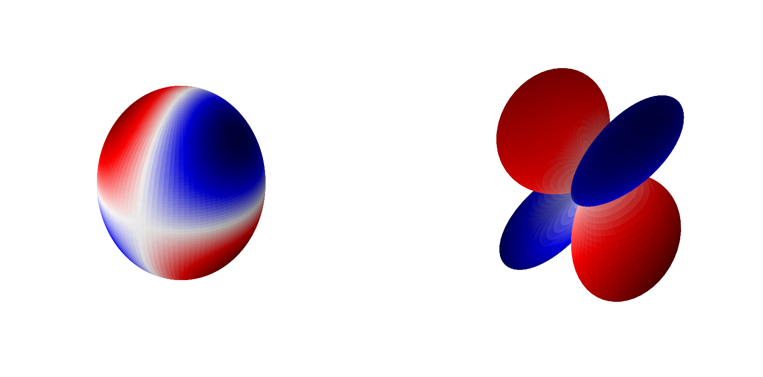
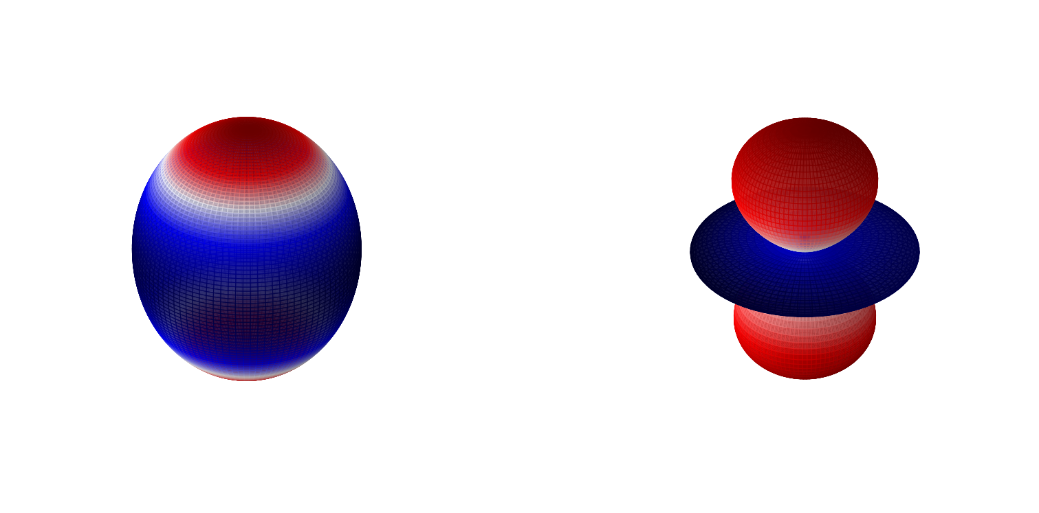
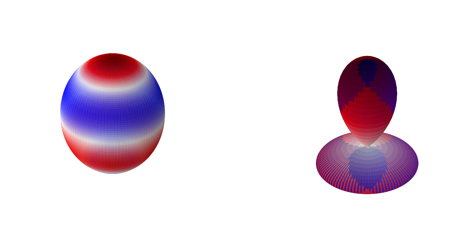
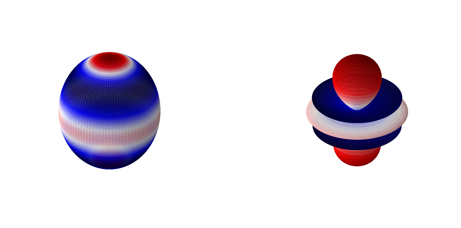
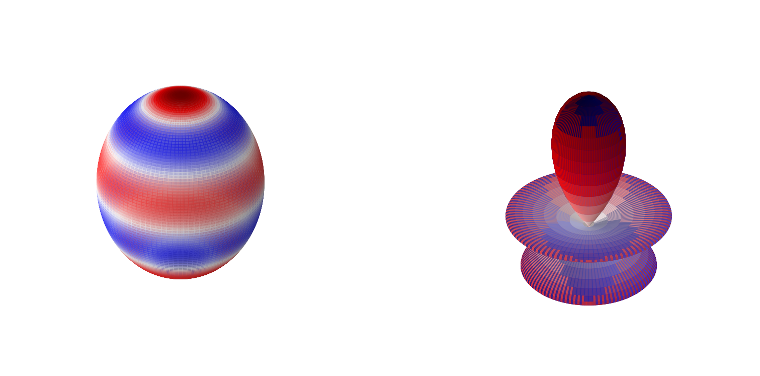
\(Y_l^m(\theta,\phi)\propto P_l^{|m|}(\cos\theta)e^{im\phi}\).

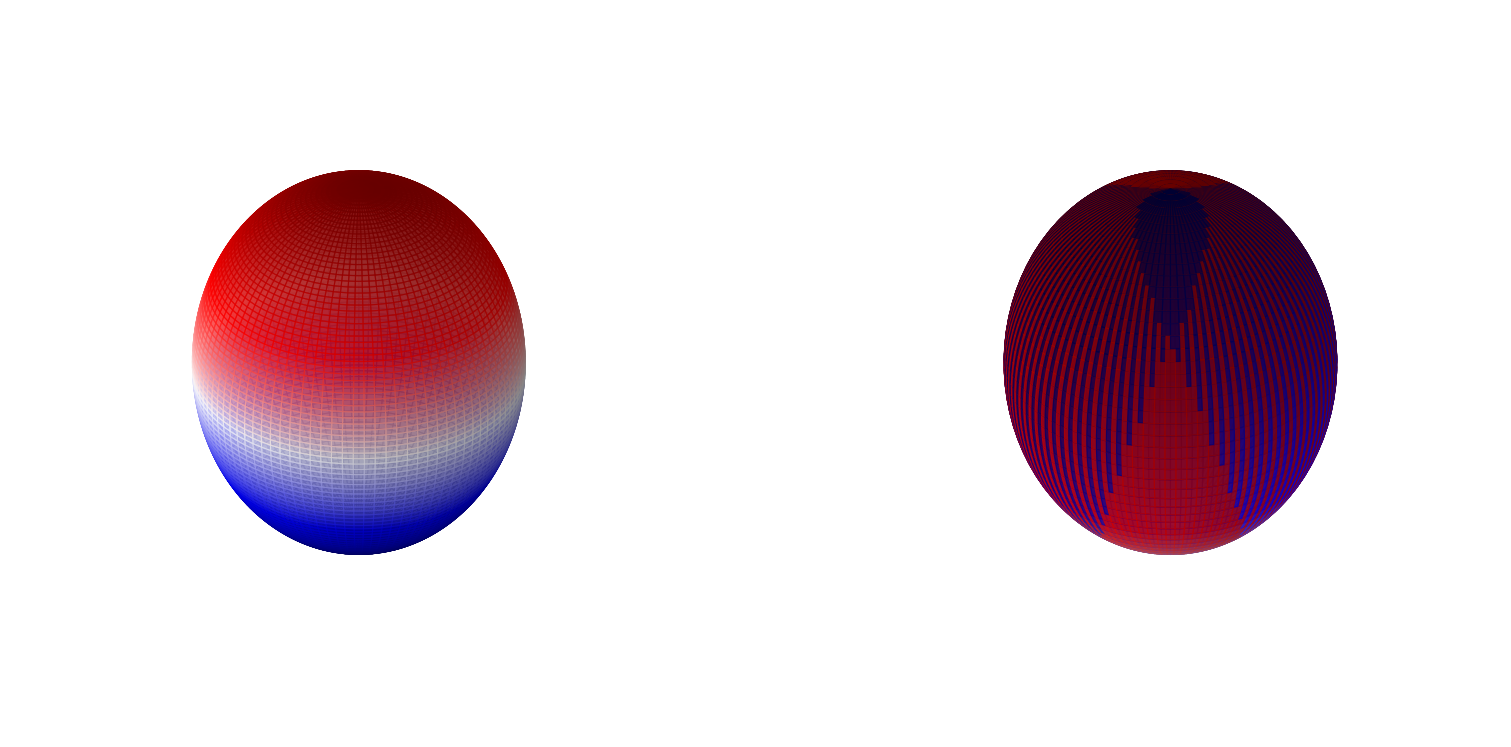
These are the spherical harmonics. We will now look at some of these.

# make two plots of the same spherical harmonic
from mpl_toolkits.mplot3d import Axes3D
from matplotlib import cm, colors
import numpy as np
import matplotlib.pyplot as plt
%matplotlib inline
from scipy.special import sph_harm
def plot_spherical_harmonic(m,l,theta=np.linspace(0,np.pi,100),phi=np.linspace(0,2*np.pi,100)):
    THETA, PHI = np.meshgrid(theta, phi)
    X = np.sin(THETA) * np.cos(PHI)
    Y = np.sin(THETA) * np.sin(PHI)
    Z = np.cos(THETA)
    # Calculate the spherical harmonic Y(l,m) and normalize to [0,1]
    fcolors = sph_harm(m, l, PHI, THETA).real
    s = sph_harm(m, l, PHI, THETA).real
    s /= s.max()
    fmax, fmin = fcolors.max(), fcolors.min()
    fcolors = (fcolors - fmin)/(fmax - fmin)
    

    # Set the aspect ratio to 1 so our sphere looks spherical
    fig = plt.figure(figsize=(24,12),dpi= 80, facecolor='w', edgecolor='k')
    ax = fig.add_subplot(1, 2, 1, projection='3d')
    ax.plot_surface(X, Y, Z,  rstride=1, cstride=1, facecolors=cm.seismic(fcolors))
    ax.set_axis_off()
    ax = fig.add_subplot(1, 2, 2, projection='3d')
    ax.plot_surface(X*s, Y*s, Z*s,  rstride=1, cstride=1, facecolors=cm.seismic(fcolors))
    # Turn off the axis planes
    ax.set_axis_off()

plt.show()

import numpy as np
import matplotlib.pyplot as plt
from scipy.special import sph_harm
%matplotlib inline

plot_spherical_harmonic(0,1)
plot_spherical_harmonic(0,2)
plot_spherical_harmonic(0,3)
plot_spherical_harmonic(0,4)
plot_spherical_harmonic(0,5)

plot_spherical_harmonic(1,2)