5.1.2. What is a Model?#
5.1.2.1. Motivation#
How do we study systems we cannot directly observe? We build models and test how those models work. Maps and weather forecasts, for examples, are models of systems or processes of which we cannot make a complete, direct observation. In Chemistry, we cannot directly observe atoms and molecules and thus must make inferences, construct models, and test the limitations of these models.
5.1.2.2. Learning Objectives#
After working through this notebook, you will be able to:
Define what is meant by a scientific model and distinguish models from theories and laws.
Explain how models are used to generate predictions and test hypotheses within the scientific method.
Identify assumptions and limitations inherent in different types of molecular models.
item Compare empirical, conceptual, and computational models used in chemistry.
5.1.2.3. Coding Concepts#
The following coding concepts are employed in this notebook:
Variables
Functions
Plotting with matplotlib
5.1.3. The Scientific Method#
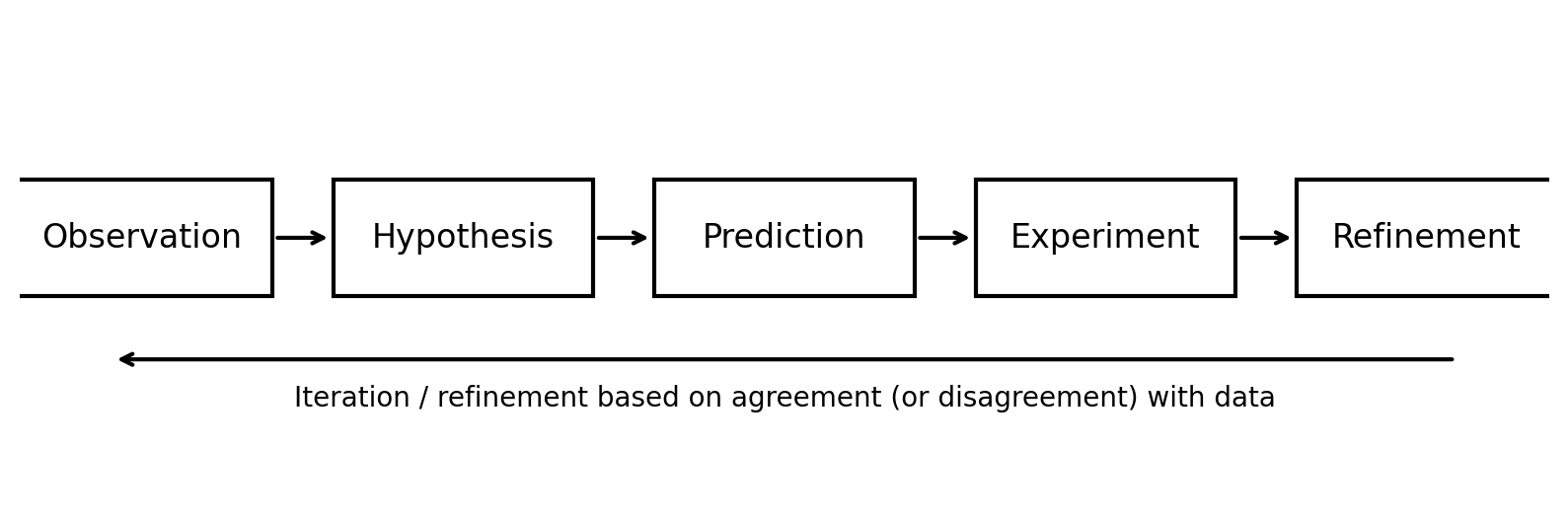
Science seeks to understand and predict natural phenomena through a systematic process known as the scientific method. While the details of this process vary across disciplines, its essential components are common to all areas of science, including chemistry. The scientific method is often summarized as a sequence of observation, hypothesis formation,prediction, experimentation, and refinement.
Show code cell source
import numpy as np
import matplotlib.pyplot as plt

# ---------- Figure 1: Scientific Method Flowchart ----------
plt.figure(figsize=(10, 3.2), dpi=200)
ax = plt.gca()
ax.set_axis_off()

steps = ["Observation", "Hypothesis", "Prediction", "Experiment", "Refinement"]
x = np.linspace(0.08, 0.92, len(steps))
y = np.full_like(x, 0.55)

# Draw boxes
for xi, label in zip(x, steps):
    ax.add_patch(plt.Rectangle((xi-0.085, y[0]-0.12), 0.17, 0.24, fill=False, linewidth=1.5))
    ax.text(xi, y[0], label, ha='center', va='center', fontsize=12)

# Arrows between boxes
for i in range(len(steps)-1):
    ax.annotate(
        "", xy=(x[i+1]-0.085, y[0]), xytext=(x[i]+0.085, y[0]),
        arrowprops=dict(arrowstyle="->", linewidth=1.5)
    )

# Iteration arrow (loop back)
ax.annotate(
    "", xy=(x[0]-0.02, 0.30), xytext=(x[-1]+0.02, 0.30),
    arrowprops=dict(arrowstyle="->", linewidth=1.5)
)
ax.text(0.5, 0.22, "Iteration / refinement based on agreement (or disagreement) with data",
        ha='center', va='center', fontsize=10)

ax.set_xlim(0, 1)
ax.set_ylim(0, 1)
plt.show();
5.1.3.1. Observation#
Scientific inquiry begins with observation. Observations may arise from direct measurement, experimental results, or patterns noticed in existing data. Importantly, observations need not be explained at the outset; their role is to identify regularities or anomalies that warrant further investigation.
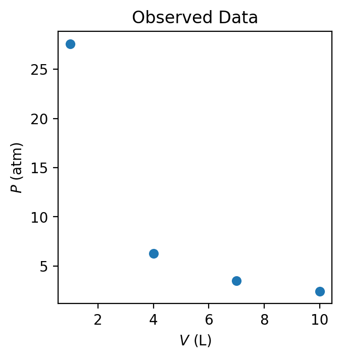
Example. Consider a set of measurements made on a fixed amount of gas contained in a sealed cylinder with a movable piston. An experimenter observes that as the volume of the gas is decreased, the measured pressure increases. Repeating the measurement at different volumes reveals a consistent inverse relationship between pressure and volume under otherwise identical conditions.
At this stage, no explanation is proposed—only the empirical relationship is noted.
Show code cell source
import numpy as np
import matplotlib.pyplot as plt


# ---------- Figure 2: Ideal Gas Prediction vs. "Real Gas" Deviations ----------
# Synthetic data: follows PV ~ constant at moderate V, deviates at small V (high density).
rng = np.random.default_rng(7)

R = 0.082057  # L·atm·mol^-1·K^-1
T = 300.0     # K
n = 1.0       # mol
PV_const = n * R * T  # ideal PV

V = np.linspace(1.0, 10.0, 4)  # liters
P_ideal = PV_const / V

# "Real gas" pressures: systematic deviation at small V + small random noise
deviation = 1 + 0.12*np.exp(-(V-1.0)/1.5)
noise = rng.normal(0, 0.015, size=V.size)
P_real = P_ideal * deviation * (1 + noise)

plt.figure(figsize=(3.5, 3.5), dpi=200)
plt.scatter(V, P_real, s=35, label="Synthetic experimental data")
plt.xlabel(r"$V\ \mathrm{(L)}$")
plt.ylabel(r"$P\ \mathrm{(atm)}$")
plt.title("Observed Data")
#plt.legend(frameon=True)
plt.show();
5.1.3.2. Hypothesis#
A hypothesis is a tentative explanation for an observed phenomenon. It is typically qualitative and framed in a way that allows it to be tested. A good hypothesis is not simply a restatement of the observation but proposes an underlying cause or mechanism.
Example. To explain the observed pressure–volume relationship, one might hypothesize that pressure arises from collisions of gas particles with the walls of the container, and that reducing the volume increases the frequency of these collisions, thereby increasing the pressure.
This hypothesis introduces an underlying mechanism but does not yet make a quantitative claim.
5.1.3.3. Prediction#
From a hypothesis, one derives predictions—specific, testable statements about what should occur under defined conditions if the hypothesis is correct. Predictions are often quantitative and allow for direct comparison with experimental results.
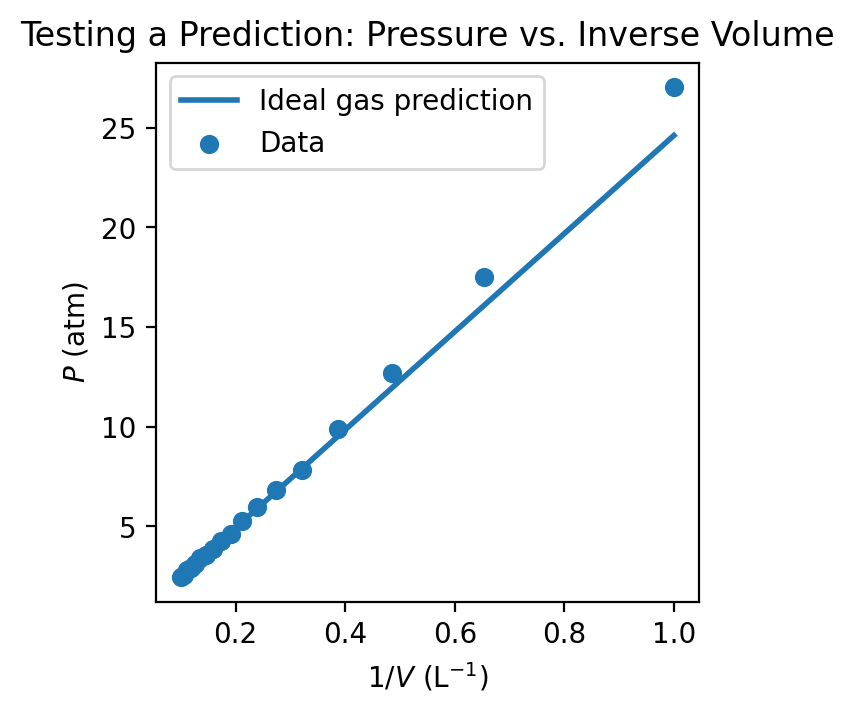
Example. From the collision-based hypothesis, one might predict that halving the volume of the gas (while keeping temperature and amount of gas constant) should approximately double the pressure. More generally, one might predict that the product of pressure and volume remains constant over a range of conditions.
Predictions transform a qualitative hypothesis into statements that can be tested.
5.1.3.4. Experiment#
Experiments are designed to test predictions by controlling relevant variables and measuring outcomes. The results of an experiment either support the predictions, contradict them, or suggest that additional factors must be considered.
Example. An experimenter systematically varies the volume of the gas while measuring the pressure, ensuring that temperature and the amount of gas remain constant. The resulting data are analyzed to determine whether the predicted inverse relationship holds and whether the product of pressure and volume remains approximately constant.
Careful experimental design is essential to ensure that the test meaningfully addresses the prediction.
Show code cell source
import numpy as np
import matplotlib.pyplot as plt


V = np.linspace(1.0, 10.0, 18)  # liters
P_ideal = PV_const / V

# "Real gas" pressures: systematic deviation at small V + small random noise
deviation = 1 + 0.12*np.exp(-(V-1.0)/1.5)
noise = rng.normal(0, 0.015, size=V.size)
P_real = P_ideal * deviation * (1 + noise)

# Plot 2A: P vs 1/V (tests linear prediction)
invV = 1.0 / V
invV_line = np.linspace(invV.min(), invV.max(), 200)
P_line = PV_const * invV_line

plt.figure(figsize=(3.5, 3.5), dpi=200)
plt.plot(invV_line, P_line, linewidth=2, label="Ideal gas prediction")
plt.scatter(invV, P_real, s=35, label="Data")
plt.xlabel(r"$1/V\ \mathrm{(L^{-1})}$")
plt.ylabel(r"$P\ \mathrm{(atm)}$")
plt.title("Testing a Prediction: Pressure vs. Inverse Volume")
plt.legend(frameon=True)
plt.show();
5.1.3.5. Refinement#
Scientific knowledge advances through refinement. When predictions agree with experiment, confidence in the hypothesis increases, but this does not imply that the explanation is complete or final. When predictions fail, the hypothesis must be revised or replaced. Refinement may involve adjusting assumptions, identifying missing variables, or developing a new conceptual framework.
Example. While the pressure-volume relationship holds under many conditions, deviations are observed at high pressures or low temperatures. These discrepancies suggest that additional factors—such as the finite size of particles or interactions between them—must be considered. The original hypothesis is therefore refined to account for these effects, leading to improved descriptions of gas behavior.
Refinement is an ongoing process, and scientific understanding evolves as new data become available.
5.1.4. The Role of Models in the Scientific Method#
A scientific model is a simplified representation of a system that captures the features relevant to a particular question. Models allow scientists to translate hypotheses into quantitative predictions that can be tested against experiment. When predictions agree with observation, confidence in the model increases; when they disagree, the model must be revised, refined, or replaced.
In chemistry, models frequently serve as the bridge between microscopic structure and macroscopic observables. For example, a model of intermolecular interactions allows one to predict boiling points, diffusion constants, or reaction rates—quantities that are directly measured in experiments but arise from molecular-scale behavior.
5.1.4.1. Models, Theories, and Laws#
It is important to distinguish between models, theories, and laws, terms that are often used interchangeably in informal discussion but have distinct meanings in scientific practice.
A law summarizes an observed regularity in nature, often in mathematical form (e.g., the ideal gas law). A theory provides a broad explanatory framework that accounts for multiple laws and observations (e.g., quantum mechanics). A model is a specific implementation or approximation derived from a theory, tailored to a particular system or question.
For example, quantum mechanics is a theory, the Schrödinger equation is a mathematical statement of that theory, and a Hartree-Fock calculation using a finite basis set is a model. Each step introduces assumptions and approximations that affect the accuracy and applicability of the results.
5.1.4.2. Types of Models in Chemistry#
Chemical models can be broadly categorized into conceptual, mathematical, and computational models, though these categories often overlap.
5.1.4.2.1. Conceptual Models#
Conceptual models provide qualitative insight into chemical behavior. Examples include Lewis structures, valence bond diagrams, and resonance structures. These models are not derived directly from first principles, but they are invaluable for building intuition about bonding, reactivity, and molecular structure.
While conceptual models are simple and easily communicated, they often lack predictive power for quantitative properties. For instance, Lewis structures cannot reliably predict reaction barriers or spectroscopic frequencies.
5.1.4.2.2. Mathematical Models#
Mathematical models express chemical behavior using equations derived from physical principles. The Schrödinger equation is a central example in chemistry, providing a formal description of electronic structure. Similarly, classical mechanics yields equations of motion that underlie molecular dynamics simulations.
Mathematical models are typically exact in form but impossible to solve analytically for systems of realistic size. As a result, further approximations are required before they can be applied in practice.
5.1.4.2.3. Computational Models#
Computational models arise when mathematical models are combined with numerical methods and approximations to produce concrete predictions. Examples include density functional theory, molecular mechanics force fields, and molecular dynamics simulations.
In computational chemistry, the term “model” often refers to the entire workflow: the choice of physical description, the approximations made, the numerical algorithms employed, and the parameters used. Different computational models may yield different predictions even when applied to the same system.
5.1.4.3. Assumptions and Approximations#
All models rely on assumptions. These assumptions determine the range of validity of the model and must be understood in order to interpret results correctly.
In quantum chemistry, common approximations include the Born-Oppenheimer separation of nuclear and electronic motion, the use of finite basis sets, and mean-field treatments of electron correlation. In molecular mechanics, electrons are not treated explicitly at all; instead, their effects are incorporated into parameterized functional forms.
Approximations are not flaws but deliberate choices. A simpler model may provide clearer insight or allow simulations of larger systems, while a more detailed model may offer higher accuracy at greater computational cost. The appropriate model depends on the scientific question being asked.
5.1.4.4. Models as Predictive Tools#
A central purpose of modeling is prediction. A useful model should make predictions that can be tested against experimental data or higher-level calculations. Agreement with experiment does not imply that a model is “true,” but rather that it is adequate for the phenomena under consideration.
For example, a molecular mechanics force field may accurately reproduce protein structures and dynamics while failing to describe chemical reactions. This limitation does not invalidate the model; it defines its domain of applicability.
5.1.4.5. Model Validation and Refinement#
When model predictions disagree with experiment, several possibilities must be considered. The model may omit important physical effects, its parameters may be inappropriate for the system under study, or the experimental conditions may not be correctly represented.
Model refinement is an iterative process. In computational chemistry, this often involves adding degrees of freedom, improving parameterization, or adopting a different theoretical framework. Throughout this process, computational results must be interpreted critically rather than accepted unconditionally.
5.1.4.6. Example: The Bohr Model of the Atom: A Case Study in Scientific Modeling#
The Bohr model of the atom provides a clear and historically important example of how scientific models function within the scientific method. Although the model is no longer considered a complete or accurate description of atomic structure, it played a crucial role in explaining experimental observations and shaping the development of modern quantum mechanics.
5.1.4.6.1. Observations: Atomic Line Spectra#
At the end of the 19th century, experiments revealed that atoms emit and absorb light at discrete wavelengths rather than continuously. When an electric discharge is passed through hydrogen gas, the emitted light consists of a series of sharp spectral lines at specific frequencies.
These discrete atomic spectra posed a serious challenge to classical physics. According to classical electrodynamics, an accelerating charged particle should continuously emit radiation. If electrons orbited the nucleus like planets around the sun, atoms would be unstable and emit a continuous spectrum—contrary to experimental observation.
5.1.4.6.2. Hypothesis: Quantized Electron Orbits#
In 1913, Niels Bohr proposed a model of the hydrogen atom based on a set of postulates rather than derivations from classical theory. In the Bohr model:
Electrons move in circular orbits around the nucleus.
Only certain orbits are allowed.
Electrons in allowed orbits do not radiate energy.
Angular momentum is quantized according to
(5.5)#\[\begin{equation} L = n\hbar \quad \text{where } n = 1, 2, 3, \dots \end{equation}\]
These assumptions were introduced to reconcile atomic stability with observed spectral lines.
Importantly, the Bohr model does not attempt to describe how or why angular momentum is quantized; it simply postulates that it is.
5.1.4.6.3. Predictions: Discrete Energy Levels#
From these assumptions, Bohr derived expressions for the allowed energies of an electron in a hydrogen atom:
The model predicts that light is emitted or absorbed when an electron transitions between two allowed energy levels. The frequency of the emitted or absorbed radiation is given by:
These expressions lead directly to the Rydberg formula for the hydrogen emission spectrum, allowing the wavelengths of spectral lines to be predicted quantitatively.
5.1.4.6.4. Experimental Validation: Agreement with Hydrogen Spectra#
The Bohr model reproduces the observed hydrogen emission spectrum exactly. The predicted wavelengths of spectral lines agree with experimental measurements, and the Rydberg constant emerges naturally from the theory.
This success provided strong evidence that atomic energy levels are quantized and demonstrated the predictive power of even a highly simplified model.
At the time, the Bohr model represented a major breakthrough in atomic physics.
5.1.4.6.5. Failure and Refinement#
Despite its success for hydrogen, the Bohr model fails when applied to more complex systems:
It does not accurately describe multi-electron atoms.
It cannot explain spectral line intensities or fine structure.
It is incompatible with classical electrodynamics.
It does not account for the wave nature of electrons.
These failures indicate that the assumptions underlying the model are incomplete. Rather than invalidating modeling as a scientific approach, these shortcomings motivated the development of a more general and accurate framework: quantum mechanics.
5.1.4.6.6. Lessons for Computational Chemistry#
The Bohr model illustrates several key ideas that recur throughout computational chemistry:
Models are simplified representations, not exact descriptions of reality.
A model can be highly successful within a limited domain of applicability.
Predictive accuracy, not realism, is the primary criterion for a useful model.
Disagreement with experiment motivates refinement rather than rejection of modeling as a whole.
Modern computational chemistry relies on a hierarchy of models—from quantum mechanical descriptions of small systems to classical simulations of large biomolecules. Like the Bohr model, each of these approaches is defined by its assumptions, strengths, and limitations.
Understanding how and why models succeed or fail is essential for interpreting computational results critically.