Basis Sets in Electronic Structure Theory

5.2.11. Basis Sets in Electronic Structure Theory#

5.2.11.1. Motivation#

In electronic structure calculations, we rarely solve the Schrödinger equation exactly. Instead, we approximate the wavefunction using a finite set of basis functions. The choice of basis set is one of the most important decisions in quantum chemistry—it directly controls accuracy, computational cost, and even qualitative conclusions.

In previous lessons, we used minimal basis sets (e.g., STO-3G) to describe molecules like H\(_2\). While these are computationally efficient, they often lack the flexibility needed to accurately describe bonding, polarization, and electron correlation.

This lesson explores how basis sets are constructed, how they are systematically improved, and how they influence calculated molecular properties.

5.2.11.2. Learning Goals#

By the end of this lesson, you should be able to:

Explain what a basis set is and why it is needed in quantum chemistry.
Distinguish between Slater-type orbitals (STOs) and Gaussian-type orbitals (GTOs).
Understand the meaning of common basis set names (e.g., STO-3G, 6-31G, cc-pVDZ).
Describe the role of:
- split-valence basis sets
- polarization functions
- diffuse functions
Predict how increasing basis set size affects energy and computational cost.
Perform and compare calculations with different basis sets in WebMO or Python.

5.2.11.3. Basis Sets/Basis Functions#

Basis functions are used throughout data science to approximate a function. Typical applications are for smoothing data or simplifying further math. The basic idea is to pick a set of functions \(\{g_i\}\) that can be used to express another function, \(f\), in an expansion. We will restrict this discussion to functions of one variable and linear coefficients in the expansion. This allows us to write \(f(x)\) as a linear combination of functions \(\{g_i(x)\}\),

\(f(x) = \sum_{i=0}^\infty c_ig_i(x)\).

This equality is only exact for certain sets of functions. This is analagous to basis sets of vector spaces. Rather than go into the details of the math of expansions and spanning spaces, we will provide two standard examples of \(\{g_i\}\)s: polynomials and gaussians.

5.2.11.3.1. Polynomial basis functions#

The idea is to express some function \(f(x)\) as a linear combination of polynomials. This is exact in the limit of infinite powers. This can be expressed as \(g_i(x) = x^i\). Thus we get

\(f(x) = \sum_{i=0}^\infty c_ix^i = c_0 + c_1x + c_2x^2 + c_3x^3...\).

If we truncate this expansion at \(i=1\) we get a linear approximation of \(f\),

\(f(x) \approx c_0 + c_1x\).

Fitting of these linear coefficients, \(c_0\) and \(c_1\), is commonly reffered to as linear regression.

5.2.11.3.2. Example: Linear Regression#

As an example of linear regression we will utilize a concoted data set and then fit these points to a line. Each “data point” represents an ordered pair \((x,f(x))\). If we have two data points we would have two depedent linear equations

\( f(x_1) = c_0 + c_1x_1 \\ f(x_2) = c_0 + c_1x_2.\)

With only two points, we can solve for \(c_0\) and \(c_1\) exactly. This simply equates to two points determine a line. Note that this can also be expressed as a matrix equation:

\(\begin{bmatrix} f(x_1) \\ f(x_2) \end{bmatrix} = \begin{bmatrix} c_0 + c_1x_1 \\ c_0 + c_1x_2 \end{bmatrix} = \begin{bmatrix} 1 & x_1 \\ 1 & x_2 \end{bmatrix} \begin{bmatrix} c_0 \\ c_1 \end{bmatrix} \).

The right-hand most expression is referred to as the coefficient matrix multiplied by the solution vector. The solution vector can be solved for by left multiplying the expression by the inverse of the coefficient matrix

\(\begin{bmatrix} c_0 \\ c_1 \end{bmatrix} = \begin{bmatrix} 1 & x_1 \\ 1 & x_2 \end{bmatrix}^{-1}\begin{bmatrix} f(x_1) \\ f(x_2)\end{bmatrix}\).

For an overdetermined set of linear equations we can solve for the solution vector (set of coefficients \(\{c_i\}\)) using a least squares algorithm. The problem is usually set up as

\(\mathbf{A}\mathbf{x} = \mathbf{b}\),

where \(\mathbf{A}\) is the coefficient matrix, \(\mathbf{x}\) is the solution vector and \(\mathbf{b}\) is the \(f(x)\) vector similar to above.

../../_images/f61699cfeccc087dbb769caeb75022143ce2b5003a2ef7696ca539ea7e332088.png

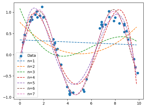
5.2.11.3.3. Example: Polynomial Regression#

We could truncate past second order to get a polynomial fit. A general Nth order polynomial approximation for \(f\) is given as

\(f(x) \approx \sum_{i=0}^N c_ix^i = c_0 + c_1x + c_2x^2 + c_3x^3 + ... + c_Nx^N\).

../../_images/433de2defcb1480ad8cf2e14415fc6c379bbbd766b0f1ebab5dbc2db52e00d5e.png

5.2.11.4. What is a Basis Set in Electronic Structure Calcualtions?#

In the Linear Combination of Atomic Orbitals (LCAO) approach, molecular orbitals are written as:

\[\psi_i = \sum_\mu c_{\mu i} \phi_\mu\]

where \(\{\phi_\mu\}\) are basis functions.

Rather than solving for an arbitrary function, we restrict the solution to a finite space spanned by these basis functions.

5.2.11.4.1. Key Idea:#

Larger/more flexible basis → more accurate wavefunction
But also → higher computational cost

5.2.11.5. STO vs GTO#

5.2.11.5.1. Slater-Type Orbitals (STOs)#

\[\phi(r) \sim e^{-\zeta r}\]

Pros:

Correct cusp at nucleus
Physically realistic decay

Cons:

Integrals are difficult to compute

5.2.11.5.2. Gaussian-Type Orbitals (GTOs)#

\[\phi(r) \sim e^{-\alpha r^2}\]

Pros:

Integrals are analytically tractable
Much faster computations

Cons:

Incorrect behavior near nucleus

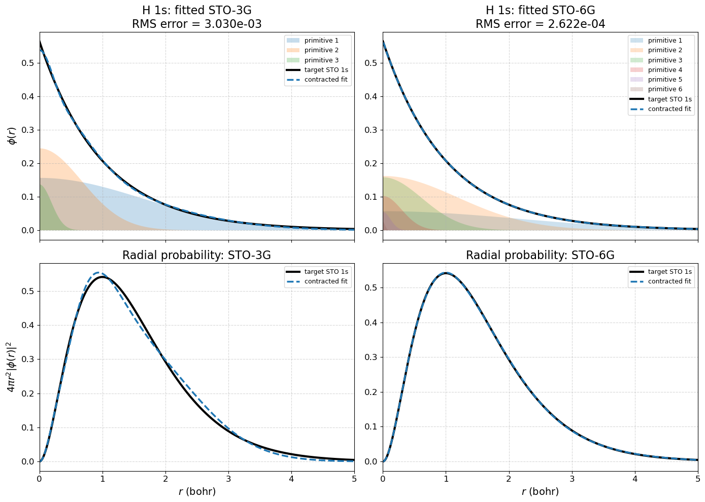
5.2.11.5.3. Solution:#

Use contracted Gaussians to approximate STOs

5.2.11.6. Minimal Basis Sets#

A minimal basis set uses one basis function per atomic orbital.

Example:

STO-3G

5.2.11.6.1. Meaning of STO-3G:#

STO: Slater-type orbital approximation
3G: each orbital is represented by 3 Gaussian functions

5.2.11.6.2. Important Clarification:#

STO-3G vs STO-6G:

Same number of orbitals
STO-6G uses more Gaussians → better approximation (not larger in dimensionality)

Show code cell source Hide code cell source

import numpy as np
import matplotlib.pyplot as plt
from scipy.optimize import least_squares

# --------------------------------------------------
# target STO and Gaussian basis functions
# --------------------------------------------------
def sto_1s(zeta, r):
    """Normalized hydrogen-like 1s Slater-type orbital."""
    return np.sqrt(zeta**3 / np.pi) * np.exp(-zeta * r)

def primitive_gaussian(alpha, r):
    """Normalized s-type primitive Gaussian."""
    return (2.0 * alpha / np.pi)**0.75 * np.exp(-alpha * r**2)

def contracted_gaussian(alphas, coeffs, r):
    """Linear combination of primitive Gaussians."""
    val = np.zeros_like(r)
    for a, c in zip(alphas, coeffs):
        val += c * primitive_gaussian(a, r)
    return val

def primitive_contributions(alphas, coeffs, r):
    """Individual primitive contributions c_i g_i(r)."""
    return [c * primitive_gaussian(a, r) for a, c in zip(alphas, coeffs)]

# --------------------------------------------------
# fitting routine
# --------------------------------------------------
def fit_sto_ng(n, zeta=1.0, rmax=6.0, npts=5000):
    """
    Fit an n-Gaussian contracted function to the STO 1s target.
    Returns exponents, coefficients, radial grid, target, fit, RMS error.
    """
    r = np.linspace(0.0, rmax, npts)
    target = sto_1s(zeta, r)

    alpha0 = np.logspace(-1, 1.5, n)
    coeff0 = np.ones(n) / n
    x0 = np.concatenate([np.log(alpha0), coeff0])

    def residuals(params):
        log_alphas = params[:n]
        coeffs = params[n:]
        alphas = np.exp(log_alphas)
        fit = contracted_gaussian(alphas, coeffs, r)
        return fit - target

    result = least_squares(residuals, x0, max_nfev=50000)

    alphas = np.exp(result.x[:n])
    coeffs = result.x[n:]

    idx = np.argsort(alphas)
    alphas = alphas[idx]
    coeffs = coeffs[idx]

    fit = contracted_gaussian(alphas, coeffs, r)
    rms = np.sqrt(np.mean((fit - target)**2))

    return alphas, coeffs, r, target, fit, rms

# --------------------------------------------------
# plotting helper
# --------------------------------------------------
def style_axis(ax, xlabel=None, ylabel=None, title=None):
    ax.grid(True, linestyle='--', alpha=0.5)
    if title is not None:
        ax.set_title(title, fontsize=16)
    if xlabel is not None:
        ax.set_xlabel(xlabel, fontsize=14)
    if ylabel is not None:
        ax.set_ylabel(ylabel, fontsize=14)
    ax.tick_params(axis='both', labelsize=12)

# --------------------------------------------------
# fit STO-3G and STO-6G numerically
# --------------------------------------------------
alpha3, coeff3, r, target, fit3, rms3 = fit_sto_ng(3, zeta=1.0)
alpha6, coeff6, _, _, fit6, rms6 = fit_sto_ng(6, zeta=1.0)

prims3 = primitive_contributions(alpha3, coeff3, r)
prims6 = primitive_contributions(alpha6, coeff6, r)

# radial probabilities
P_target = 4.0 * np.pi * r**2 * target**2
P_fit3   = 4.0 * np.pi * r**2 * fit3**2
P_fit6   = 4.0 * np.pi * r**2 * fit6**2

# --------------------------------------------------
# make 2x2 figure
# --------------------------------------------------
fig, axes = plt.subplots(2, 2, figsize=(14, 10), sharex='col')

# ---------------- top-left: STO-3G wavefunction ----------------
ax = axes[0, 0]
style_axis(
    ax,
    ylabel=r"$\phi(r)$",
    title=f"H 1s: fitted STO-3G\nRMS error = {rms3:.3e}"
)

for i, p in enumerate(prims3, start=1):
    ax.fill_between(r, 0.0, p, alpha=0.25, label=f"primitive {i}")

ax.plot(r, target, color='black', lw=3, label="target STO 1s")
ax.plot(r, fit3, color='tab:blue', lw=2.5, ls='--', label="contracted fit")
ax.set_xlim(0, 5)
ax.legend(fontsize=9, loc="best")

# ---------------- top-right: STO-6G wavefunction ----------------
ax = axes[0, 1]
style_axis(
    ax,
    title=f"H 1s: fitted STO-6G\nRMS error = {rms6:.3e}"
)

for i, p in enumerate(prims6, start=1):
    ax.fill_between(r, 0.0, p, alpha=0.22, label=f"primitive {i}")

ax.plot(r, target, color='black', lw=3, label="target STO 1s")
ax.plot(r, fit6, color='tab:blue', lw=2.5, ls='--', label="contracted fit")
ax.set_xlim(0, 5)
ax.legend(fontsize=9, loc="best")

# ---------------- bottom-left: STO-3G probability ----------------
ax = axes[1, 0]
style_axis(
    ax,
    xlabel=r"$r$ (bohr)",
    ylabel=r"$4\pi r^2 |\phi(r)|^2$",
    title="Radial probability: STO-3G"
)

ax.plot(r, P_target, color='black', lw=3, label="target STO 1s")
ax.plot(r, P_fit3, color='tab:blue', lw=2.5, ls='--', label="contracted fit")
ax.set_xlim(0, 5)
ax.legend(fontsize=9, loc="best")

# ---------------- bottom-right: STO-6G probability ----------------
ax = axes[1, 1]
style_axis(
    ax,
    xlabel=r"$r$ (bohr)",
    title="Radial probability: STO-6G"
)

ax.plot(r, P_target, color='black', lw=3, label="target STO 1s")
ax.plot(r, P_fit6, color='tab:blue', lw=2.5, ls='--', label="contracted fit")
ax.set_xlim(0, 5)
ax.legend(fontsize=9, loc="best")

plt.tight_layout()
plt.show()

../../_images/b611683ca3fb858031e73c7424741c1ba79fa48e1a6552ee5858a2c7887ce15e.png

5.2.11.7. Split-Valence (aka double zeta) Basis Sets#

Minimal basis sets are too rigid, especially for valence electrons.

5.2.11.7.1. Idea:#

Use multiple functions to describe valence orbitals.

A common nomenclature for these basis is, e.g 6-31G. These are called Pople basis sets. 6-31G means that each core orbital is approximated by a single “6”-contracted Gaussian basis funciton while each valence oribtal is split into two basis funcitons, one that is a “3”-contracted Gaussian function and another that is a single Gaussian.

Example 1: 6-31G

Core orbitals: 6 Gaussians
Valence orbitals:
- 3 Gaussians (inner part)
- 1 Gaussian (outer part)

Example 2: 3-21G

Core orbitals: 3 Gaussians
Valence orbitals:
- 2 Gaussians (inner part)
- 1 Gaussian (outer part)

5.2.11.7.2. Why?#

Allows orbitals to expand/contract during bonding

5.2.11.7.3. Example: A Carbon Atom in 6-31G#

Carbon has 1 core spatial orbital: The 1s orbital is approximated as a single basis function (which is a 6 Gaussian contraction)
Carbon has 4 valence orbitals:
- 2s obital is approximated by 2 functions: A 3 Gaussian contraction inner part and a 1 Gaussian outer part
- 3 2p orbitals each approximation by 2 functions: A 3 Gaussian contraction inner part and a 1 Gaussian outer part
Carbon has 1 + 4*2 = 9 basis functions

5.2.11.7.4. Triple Zeta Basis Sets#

Even double zeta basis sets are sometimes not flexible enough to describe the valence orbitals.

5.2.11.7.5. Idea:#

Add another basis function to the valence orbitals. In the Pople nomenclature, these look like, e.g. 6-311G.

Example 1: 6-311G

Core orbitals: 6 Gaussians
Valence orbitals:
- 3 Gaussians (inner part)
- 1 Gaussian (outer part)
- 1 Gaussian (outer part)

5.2.11.7.6. Example A Carbon Atom in 6-311G#

Carbon has 1 core spatial orbital: The 1s orbital is approximated as a single basis function (which is a 6 Gaussian contraction)
Carbon has 4 valence orbitals:
- 2s obital is approximated by 2 functions: A 3 Gaussian contraction inner part, a 1 Gaussian outer part, and another a 1 Gaussian outer part
- 3 2p orbitals each approximation by 2 functions: A 3 Gaussian contraction inner part, a 1 Gaussian outer part, and another a 1 Gaussian outer part
Carbon has 1 + 4*3 = 13 basis functions in 6-311G basis

5.2.11.8. Polarization Functions#

Polarization functions allow orbitals to change shape.

Example:

Add d-functions to carbon
Add p-functions to hydrogen

Notation:

6-31G(d)
6-31G(d,p)

5.2.11.8.1. Physical Meaning:#

Enables directional bonding
Critical for:
- molecular geometry
- reaction barriers

5.2.11.8.2. Example: A Carbon Atom in 6-31G(d)#

Carbon has 1 core spatial orbital: The 1s orbital is approximated as a single basis function (which is a 6 Gaussian contraction)
Carbon has 4 valence orbitals:
- 2s obital is approximated by 2 functions: A 3 Gaussian contraction inner part and a 1 Gaussian outer part
- 3 2p orbitals each approximation by 2 functions: A 3 Gaussian contraction inner part and a 1 Gaussian outer part
We add 6 d-like functions (should be five but mathematically easier to add six)
Carbon has 1 + 4*2 + 6 = 15 basis functions

5.2.11.9. Diffuse Functions#

Diffuse functions describe electrons far from the nucleus.